
Predicting fishing effort in Micronesia
fishing_prediction.RmdWe will create a Generalized Additive Model (GAM) of fishing effort
in the Exclusive Economic Zone (EEZ) of the Federated States of
Micronesia (FSM), using physical and environmental predictors obtained
using the oceandatr package, illustrating the usefulness of
oceandatr for retrieving, gridding, and transforming
spatial data with minimal input from the user. Note that this vignette
is not intended as a guide to GAMs - entire books are written about
that.
Obtain a spatial boundary for the area of interest
Download FSM’s EEZ using oceandatr
fsm <- get_boundary("Micronesia")
#> Cache is fresh. Reading: '/tmp/RtmpmxUBrw/eez-9e33e424/eez.shp'
#> (Last Modified: 2026-07-03 10:22:32.424902)

plot(fsm[,1], axes = T)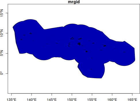
Federated States of Micronesia’s EEZ
Get a suitable coordinate reference system for the area
The ocean boundary comes in the widely used, ‘unprojected’, coordinate reference system (CRS) EPSG:4326. We will use a local, equal-area projection, which we can find using the Projection Wizard website, entering the geographic extent of the EEZ:
(geog_extent <- sf::st_bbox(fsm))
#>       xmin       ymin       xmax       ymax
#> 135.315556  -1.171389 165.676111  13.440706
So the North extent coordinate is 14, South extent is -2, East extent is 166 E, and the West extent is 135 E. Putting this information in Projection Wizard and clicking the “PROJ” link underneath the map, we get a suitable equal-area projection.
fsm_proj <- "+proj=cea +lon_0=150.5 +lat_ts=7 +datum=WGS84 +units=m +no_defs"

# project the EEZ boundary into the local CRS
fsm_eez_proj <- fsm |>
  sf::st_transform(fsm_proj) |>
  vect() #convert to a SpatVector for easy plotting with the rasters
Create a raster grid for our data
We can now create the grid we will use for all our data. The grid cell size is set at 10 km to ensure that the model runs reasonably fast; smaller grid cell sizes will result in more cells, and hence more data in the model.
fsm_grid <- get_grid(fsm, resolution = 10e3, crs = fsm_proj)Fishing effort data
We can now retrieve gridded fishing effort data for FSM from Global
Fishing Watch. As noted in the help file (?get_gfw()), you
need a (free) API key from Global Fishing Watch for this to work. For
simplicity, we will use the mean total annual effort in each grid cell,
using data from 2024 and 2025. In a more detailed model setup, different
fishing gears, such as purse seine and longlines, could be modelled
separately, and time could be included as a factor in the model.
fishing_effort <- get_gfw(fsm_grid,
                          start_year = 2024,
                          end_year = 2025,
                          group_by = "location",
                          summarise = "mean_total_annual_effort")
#> GFW data already downloaded, using cached version

plot(log(fishing_effort+1))
lines(fsm_eez_proj, col = "orange", lwd = 0.5)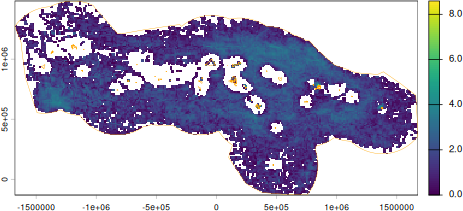
Mean annual fishing effort. 2024 - 2025
We plot the log+1 transformed data because there are many zero or near zero values.
Mask fishing effort nearshore
There are some anomalously high values close to the islands. No industrial fishing is allowed within 12nm of shore in FSM, so to remove these missclassified values we can download FSM’s 12nm polygons and mask the fishing effort data.
fsm_12nm <- get_boundary("Micronesia", type = "12nm") |>
  sf::st_transform(fsm_proj)
#> Cache is fresh. Reading: '/tmp/RtmpmxUBrw/eez_12nm-77146a5e/eez_12nm.shp'
#> (Last Modified: 2026-07-03 10:23:23.333102)

fishing_effort_masked <- mask(fishing_effort, mask = fsm_12nm, inverse = TRUE)

plot(log(fishing_effort_masked+1))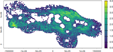
Mean annual fishing effort with nearshore values removed.
Retrieve predictor data
Bathymetry and environmental conditions, such as temperature,
chlorophyll concentration, and dissolved oxygen, are all known to the be
predictors of fish distributions. Distance from port is also a known
factor in predicting fishing effort. We will use these variables as
predictors of fishing effort in our simple model. All the data is
downloaded, gridded, and transformed to the correct CRS using
oceandatr.
# seafloor depth
bathy <- get_bathymetry(spatial_grid = fsm_grid,
                        classify_bathymetry = FALSE)
#> Bathymetry data already downloaded, loading data from: /tmp/RtmpmxUBrw/bathy_135.32_165.68_-1.17_13.44.tif

# distance to ports data
dist_port <- get_dist(spatial_grid = fsm_grid,
                      dist_to = "ports")

# sea surface environmental data such as temperature and chlorophyll
enviro_data <- get_enviro_zones(fsm_grid,
                                enviro_zones = FALSE)
#> Retrieving environmental data from https://erddap.bio-oracle.org/erddap/, or disk if previously downloaded.
#> Data retrieval complete
Model
We will use a basic Generalized Additive Model (GAM), implemented
using the mgcv R package. First we create a multi-layer
raster with all the data we want to use in the model, in our case:
Response variable:
- Fishing effort (log+1 transformed)
Predictor variables:
- Seafloor depth
- Distance to port
- Mean sea surface temperature
- Dissolved oxygen
#create multi-layer raster with all data needed for modelling
model_data <- c(log(fishing_effort_masked+1),
                bathy,
                dist_port,
                enviro_data[[c("Mean_temp", "Dissolved_oxygen")]]) |>
  mask(fsm_12nm, inverse = TRUE)


plot(model_data, main = c("Fishing effort", "Seafloor depth", "Distance to port", "Mean SST", "Dissolved oxgen"))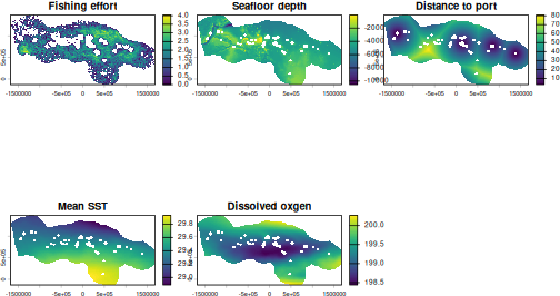
Data for GAM
These data are then converted to a data frame for the modelling process.
# convert the raster to a dataframe
model_df <- model_data |>
  as.data.frame(xy = TRUE, na.rm = TRUE)
Now we can fit a basic GAM, using the gam() function from the package mgcv. Predictor variables (seafloor depth, distance to port, SST and dissolved oxygen) are modelled using penalized thin-plate regression splines, while a geographic Gaussian process smoother is included to account for spatial dependency across the pelagic grid. The model is fitted via Restricted Maximum Likelihood (REML) estimation using the log+1 transformed response (fishing effort) variable to address data skewness and stabilize residual variance, and a normal error structure is used.
#fit the GAM
fishing_model <- mgcv::gam(
  mean_total_annual_effort ~
    s(bathymetry) +
    s(dist_ports) +
    s(Mean_temp) +
    s(Dissolved_oxygen) +
    s(x,y, bs = "gp"),
  data = model_df,
  method = "REML"
)

(model_summary <- summary.gam(fishing_model))
#>
#> Family: gaussian
#> Link function: identity
#>
#> Formula:
#> mean_total_annual_effort ~ s(bathymetry) + s(dist_ports) + s(Mean_temp) +
#>     s(Dissolved_oxygen) + s(x, y, bs = "gp")
#>
#> Parametric coefficients:
#>             Estimate Std. Error t value Pr(>|t|)
#> (Intercept)  1.42992    0.00345   414.5   <2e-16 ***
#> ---
#> Signif. codes:  0 '***' 0.001 '**' 0.01 '*' 0.05 '.' 0.1 ' ' 1
#>
#> Approximate significance of smooth terms:
#>                        edf Ref.df      F p-value
#> s(bathymetry)        8.461  8.922  18.41  <2e-16 ***
#> s(dist_ports)        8.711  8.977  61.78  <2e-16 ***
#> s(Mean_temp)         8.892  8.995  99.89  <2e-16 ***
#> s(Dissolved_oxygen)  8.593  8.957  35.27  <2e-16 ***
#> s(x,y)              31.332 31.847 330.51  <2e-16 ***
#> ---
#> Signif. codes:  0 '***' 0.001 '**' 0.01 '*' 0.05 '.' 0.1 ' ' 1
#>
#> R-sq.(adj) =   0.49   Deviance explained = 49.1%
#> -REML =  18902  Scale est. = 0.28241   n = 23726
The model successfully captured the spatial distribution of fishing effort (adjusted R2 = 0.490) and all predictor variables had highly significant, non-linear effects (p < 0.001)
We can predict fishing effort using the GAM for the same model grid we used as input, and compare the GFW data to the predictions.
# Predict using the GAM
model_df$predicted_effort <- mgcv::predict.gam(fishing_model)

# Convert back to a raster for mapping
pred_rast <- rast(model_df[, c("x", "y", "predicted_effort")], crs = fsm_proj)

#plot GFW data and predictions next to each other
par(mfrow = c(1,2))
plot(log(fishing_effort_masked+1), main = "Global Fishing Watch")
plot(pred_rast, main = "Model predictions ")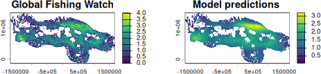
Model prediction compared to GFW data
Not bad for a very rough GAM!
When building a more robust model, diagnostic plots and information
should be examined, e.g. using
mgcv::plot.gam(fishing_model) and
mgcv::gam.check(fishing_model).