Gridding spatial data • oceandatr

Apart from oceandatr’s for retrieving data from specific datasets, such as get_seamounts(), there are three generic functions:

get_boundary(): retrieves the boundaries for a marine or terrestrial area, such as a country or Exclusive Economic Zone (EEZ)
get_grid(): creates a spatial grid
get_data_in_grid(): grids spatial data; can also be used to crop/ intersect a polygon with data

This vignette show how to use these functions for get gridded data, in terra::rast and sf format, using the EEZ’s of Samoa and Fiji as examples.

#load the package
library(oceandatr)
library(oceandatrsets)

Get a boundary

We can obtain grids in raster (terra::rast) or vector (sf) format. First we need a polygon that we want to create a grid for. We can retrieve boundaries for countries, Exclusive Economic Zones (EEZs), oceans, and several other jurisdiction types using get_boundary(). In this example we will get the EEZ for the Pacific nation of Samoa.

#get Samoa's EEZ
samoa_eez <- get_boundary(name = "Samoa")

plot(samoa_eez["geometry"], axes = TRUE)

Get a grid

We also need to provide a suitable projection for the area we are interested in. Projection Wizard is useful for this purpose. For spatial planning, equal area projections are normally best. A good option for the Pacific is EPSG:8859, which is equal area and centered on the Pacific.


# Create a raster grid with 10km sized cells
samoa_grid <- get_grid(boundary = samoa_eez, resolution = 10000, crs = 8859)

#plot the grid
terra::plot(samoa_grid)
terra::lines(terra::as.polygons(samoa_grid, dissolve = FALSE)) #add the outlines of each cell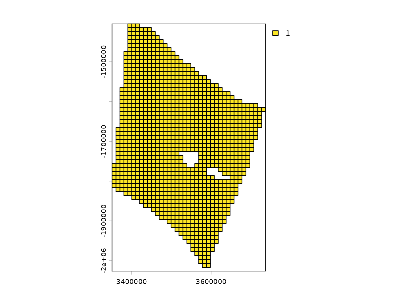

To obtain a grid in sf format we can use arguments option = "sf_square" or option = "sf_hex" in get_grid to specify square or hexagonal cells. We will create and plot a hexagonal grid with 10 km wide cells.

samoa_grid_sf <- get_grid(boundary = samoa_eez, resolution = 10000, crs = 8859, output = "sf_hex")

plot(samoa_grid_sf)

Grid data

Now we can grid some data. Data can be in raster (terra::rast) or sf format. Here’s an example using a global map of seafloor ridges which is in sf format and is part of the oceandatrsets package that houses datasets for oceandatr:

# ridges data for area of Pacific
ridges <- readRDS(system.file("extdata/geomorphology", "ridges.rds", package = "oceandatrsets"))

#grid the data
ridges_gridded <- get_data_in_grid(spatial_grid = samoa_grid, dat = ridges)

#plot
terra::plot(ridges_gridded)
terra::lines(samoa_eez |> sf::st_transform(crs = 8859)) #add Samoa's EEZ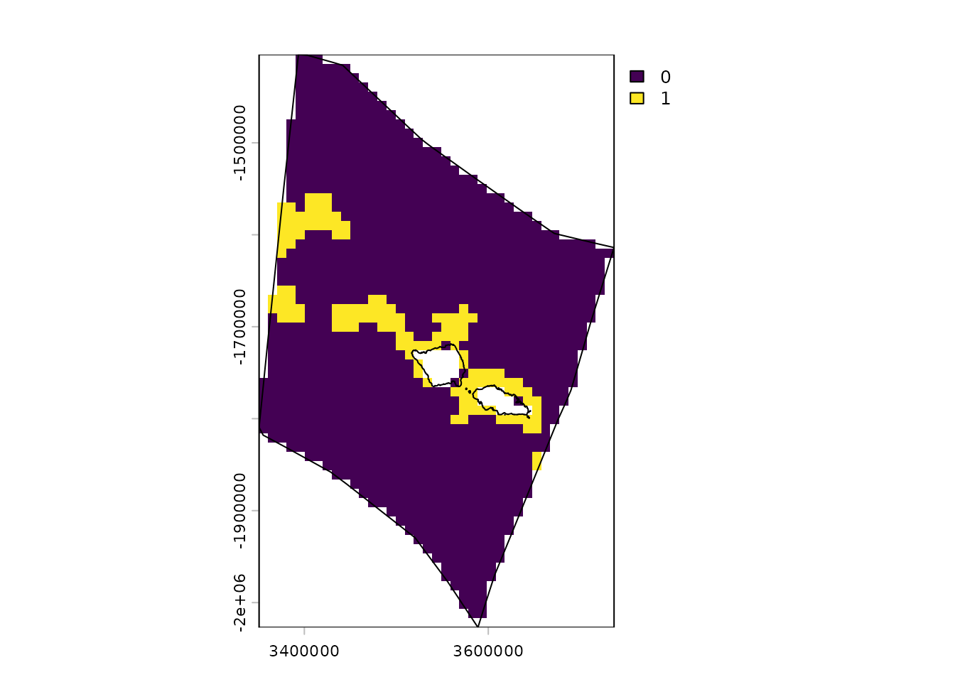

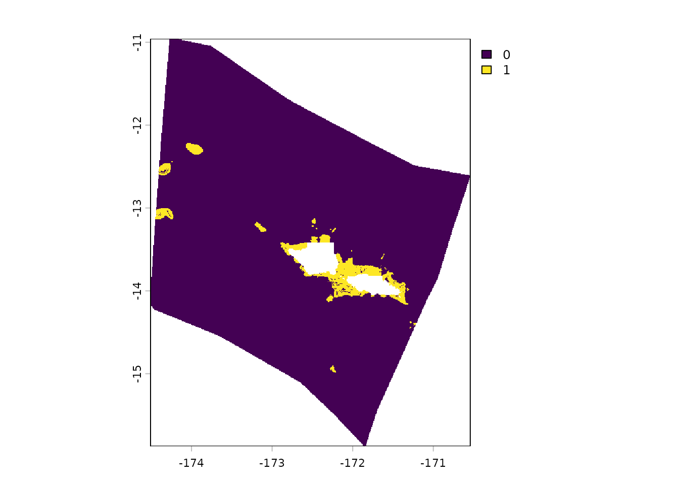
And another example using raster data, in this case global cold water coral distribution data

#load cold water coral data
cold_coral <- terra::rast(system.file("extdata", "cold_coral.tif", package = "oceandatrsets"))

#grid the data
coral_gridded <- get_data_in_grid(spatial_grid = samoa_grid, dat = cold_coral)

#plot
terra::plot(coral_gridded)
terra::lines(samoa_eez |> sf::st_transform(crs = 8859)) #add Samoa's EEZ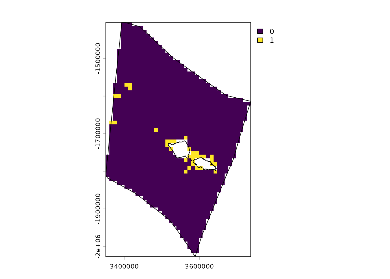

We can also use the sf grid we created to return gridded data in sf format:

#grid the data
ridges_gridded_sf <- get_data_in_grid(spatial_grid = samoa_grid_sf, dat = ridges)

#plot
plot(ridges_gridded_sf)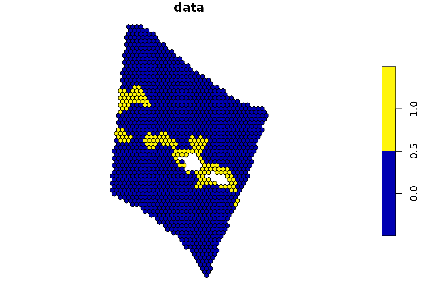

We can also grid sf data that contains multiple data features, such as habitat types. To do this, we provide the name of the column that contains the names of the features we want to grid as the feature_names argument in get_data_data_in_grid(). This creates a multi-layer grid. For raster data this means multiple raster layers and for sf grids multi-column objects. Here’s an example using sf data that classifies the worlds abyssal oceans into 3 categories:

#load the data
abyssal_features <- system.file("extdata", "abyssal_classes_pacific.rds", package = "oceandatr") |>
  readRDS()

#grid the data
abyssal_features_sf <- get_data_in_grid(spatial_grid = samoa_grid_sf, dat = abyssal_features, feature_names = "Class")

#plot
plot(abyssal_features_sf)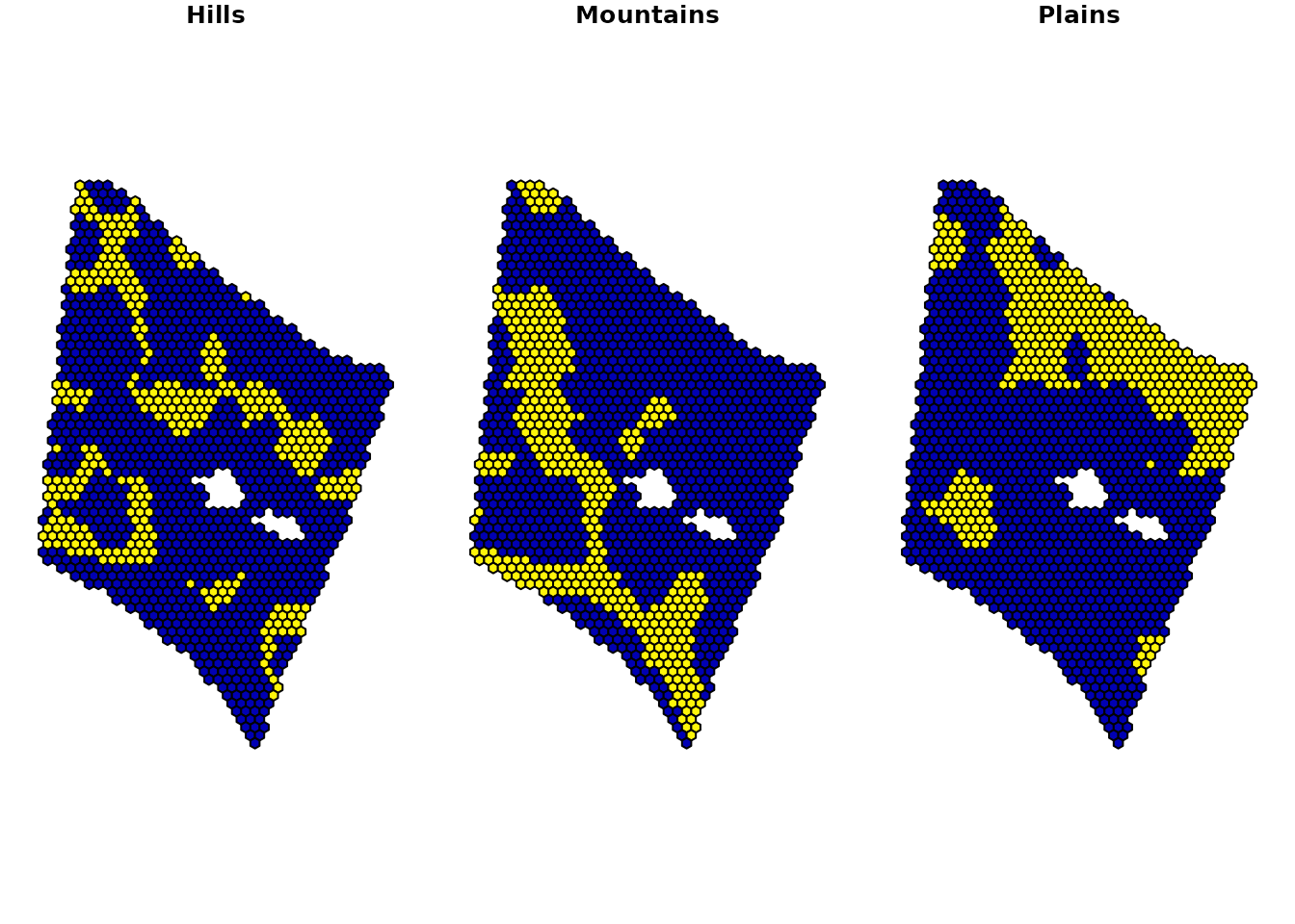

oceandatr also works with grids that cross the antimeridian (international date line). You can set antimeridian = TRUE in get_data_in_grid if you know you are using a grid that crosses the antimeridian, or if antimeridian = NULL (the default option), the function will automatically determine if the grid crosses the antimeridian. Here’s an example using Fiji’s EEZ as the grid area.

#load the Fiji EEZ polygon
fiji_eez <- get_boundary(name = "Fiji")

#create a grid for the Fiji EEZ
fiji_grid <- get_grid(boundary = fiji_eez, resolution = 20000, crs = 8859, output = "sf_square")

#get abyssal plains classification for Fiji grid
fiji_abyssal_features <- get_data_in_grid(spatial_grid = fiji_grid, dat = abyssal_features, feature_names = "Class")

#plot
plot(fiji_abyssal_features, border = FALSE)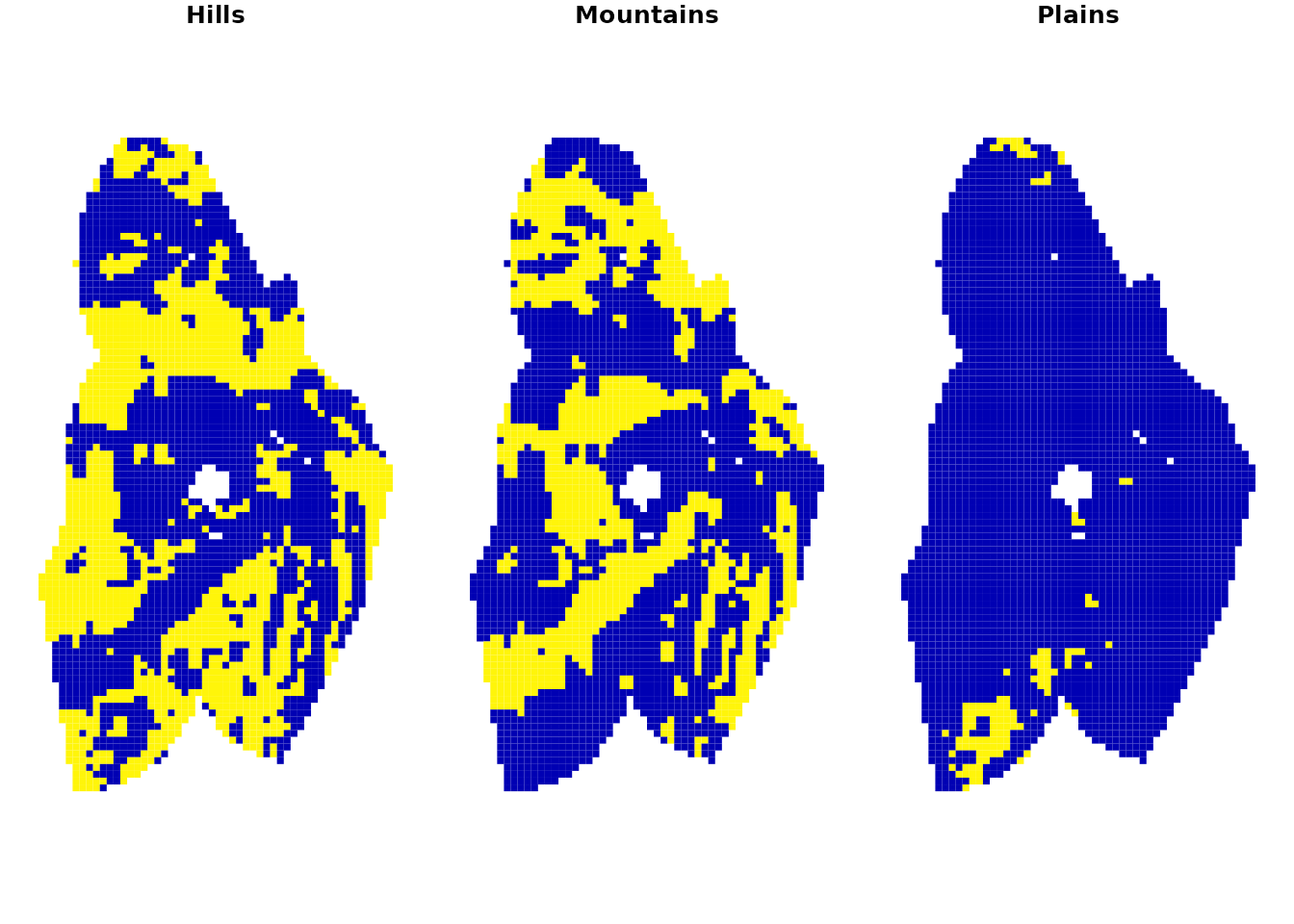

Get raw data

If you just want to get data for an area, but don’t want to grid it, you can provide an sf polygon to get_data_in_grid() and set raw = TRUE.

fiji_abyssal_features_raw <- get_data_in_grid(spatial_grid = fiji_eez, dat = abyssal_features, raw = TRUE)

#shift longitude to make it easier to view data
plot(fiji_abyssal_features_raw[1] |> sf::st_shift_longitude(), border = FALSE)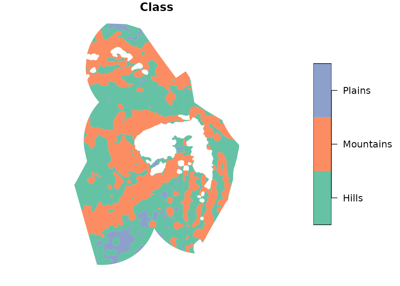

samoa_coral_raw <- get_data_in_grid(spatial_grid = samoa_eez, dat = cold_coral, raw = TRUE)

terra::plot(samoa_coral_raw)