Get distance to port or shore for a spatial grid

Calculates distance from shore, port or anchorage for each grid cell in the provided spatial grid. Spatial grid can be terra::rast() or sf format.

Usage

get_dist(
  spatial_grid,
  dist_to = "shore",
  raw = FALSE,
  inverse = FALSE,
  name = NULL,
  antimeridian = NULL
)

Arguments

spatial_grid: sf or terra::rast() grid, e.g. created using get_grid(). Alternatively, if raw data is required, an sf polygon can be provided, e.g. created using get_boundary(), and set raw = TRUE.
dist_to: character which data to use to calculate distance to. Default is "shore" (Natural Earth land polygons); other possible values are "ports" (WPI Ports), "anchorages_land_masked", "anchorages_grouped" and "anchorages_all" (GFW anchorages).
raw: logical set to TRUE to retrieve the raw shore, port or anchorage data within the extent of the spatial_grid. Note that the closest shore, port or anchorage may be outside the extent.
inverse: logical set to TRUE to get the inverse of distance, i.e. highest values become lowest and vice versa. Can be useful if the result is to be used as a proxy for fishing activity, where the closer a grid cell is to the port or shore, the more fishing activity there might be. Default is FALSE.
name: string; name of raster or column in sf object that is returned
antimeridian: Does spatial_grid span the antimeridian? If so, this should be set to TRUE, otherwise set to FALSE. If set to NULL (default) the function will try to check if spatial_grid spans the antimeridian and set this appropriately.

Value

a terra::rast or sf object (same type as spatial_grid input) with distance to shore for each grid cell.

Shore

The Natural Earth high resolution land polygons are used as the shoreline and are downloaded from the Natural Earth website (https://www.naturalearthdata.com/downloads/10m-physical-vectors/), so an internet connection is required.

Ports

Port locations are downloaded directly from the World Port Index (Pub 150): https://msi.nga.mil/Publications/WPI.

Anchorages

The anchorages data is from Global Fishing Watch and identifies anchorages as anywhere vessels with AIS remain stationary for 12 hours or more (see https://globalfishingwatch.org/datasets-and-code-anchorages/). This results in a very large number of points (~167,000). Calculating distance from all these points to each grid cell is computationally expensive. Anchorages close together have the same names, so to reduce the number of anchorages, they are aggregated by iso3 code (country code) and label (name) and the mean longitude and latitude coordinates obtained to get one anchorage point per name in each country. This data can be used by specifying dist_to = "anchorages_grouped".

To further reduce the number of points, anchorages within countries' land boundaries, e.g. along rivers, can be removed. I do this by buffering the Natural Earth land boundaries by 10km inland so as to avoid cutting off coastal anchorages that fall within the land boundary, due to inaccuracies in the Natural Earth land boundaries, e.g. for islands and other small scale coastlines, and then masking points that fall within the resulting polygons. This data can be used by specifying dist_to = "anchorages_land_masked".

The full anchorages dataset can be used by specifying dist_to = "anchorages_all", but this option may take a long time to calculate and/ or cause your system to hang.

Examples

# Get some EEZ data first 
fiji_eez <- get_boundary(name = "Fiji")
# Get a raster spatial grid for Fiji
fiji_grid <- get_grid(boundary = fiji_eez, crs = 32760, resolution = 20000)
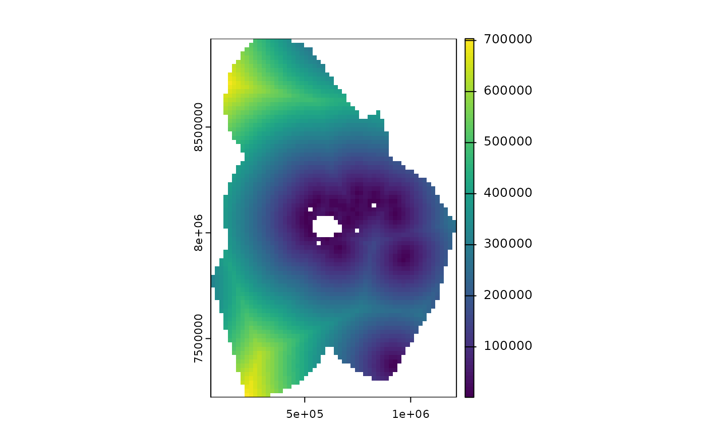
#get distance from shore for each cell in the raster
dist_from_shore_rast <- get_dist(fiji_grid)
terra::plot(dist_from_shore_rast)


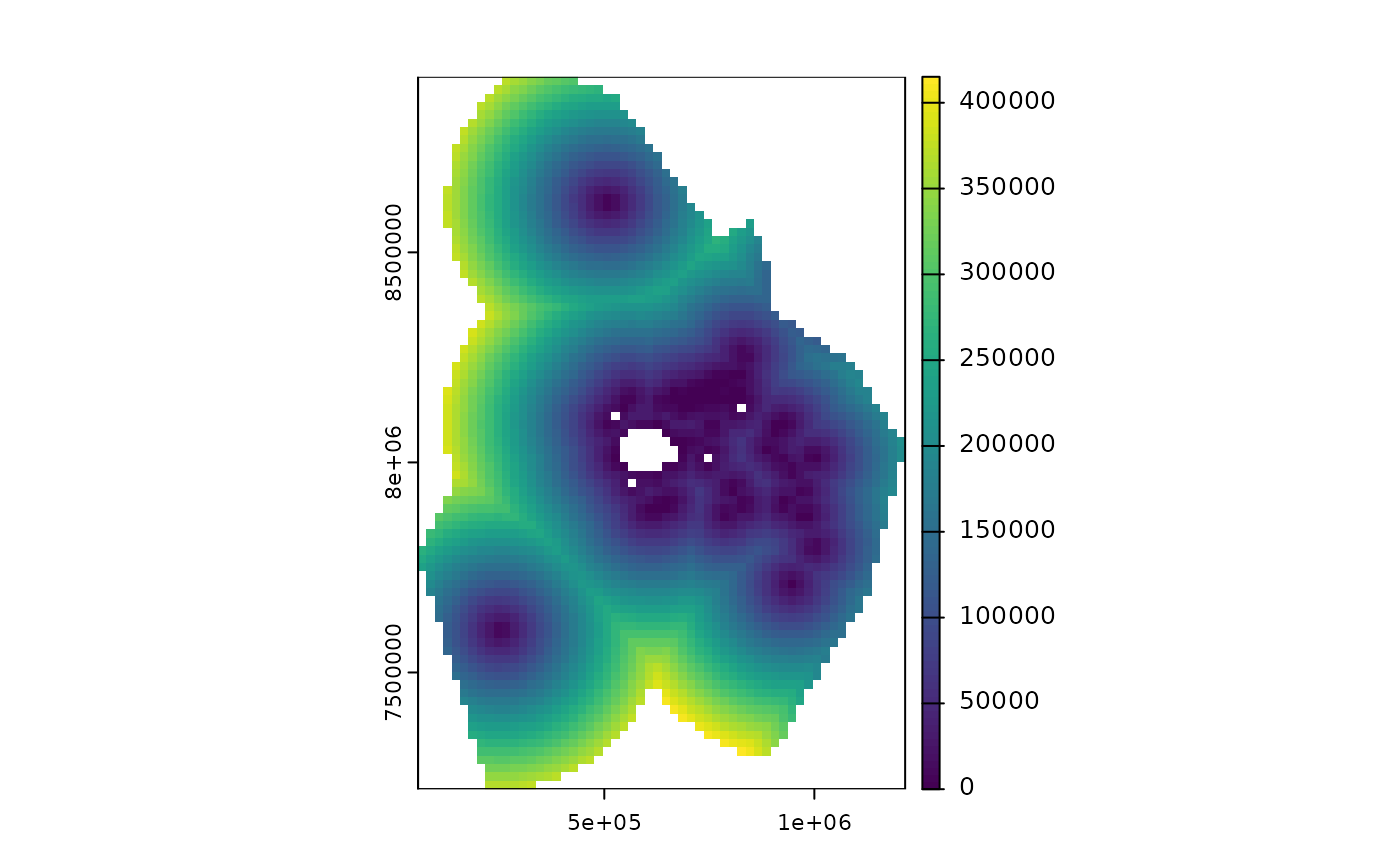#get distance to ports
dist_ports <- get_dist(fiji_grid, dist_to = "ports")
terra::plot(dist_ports)


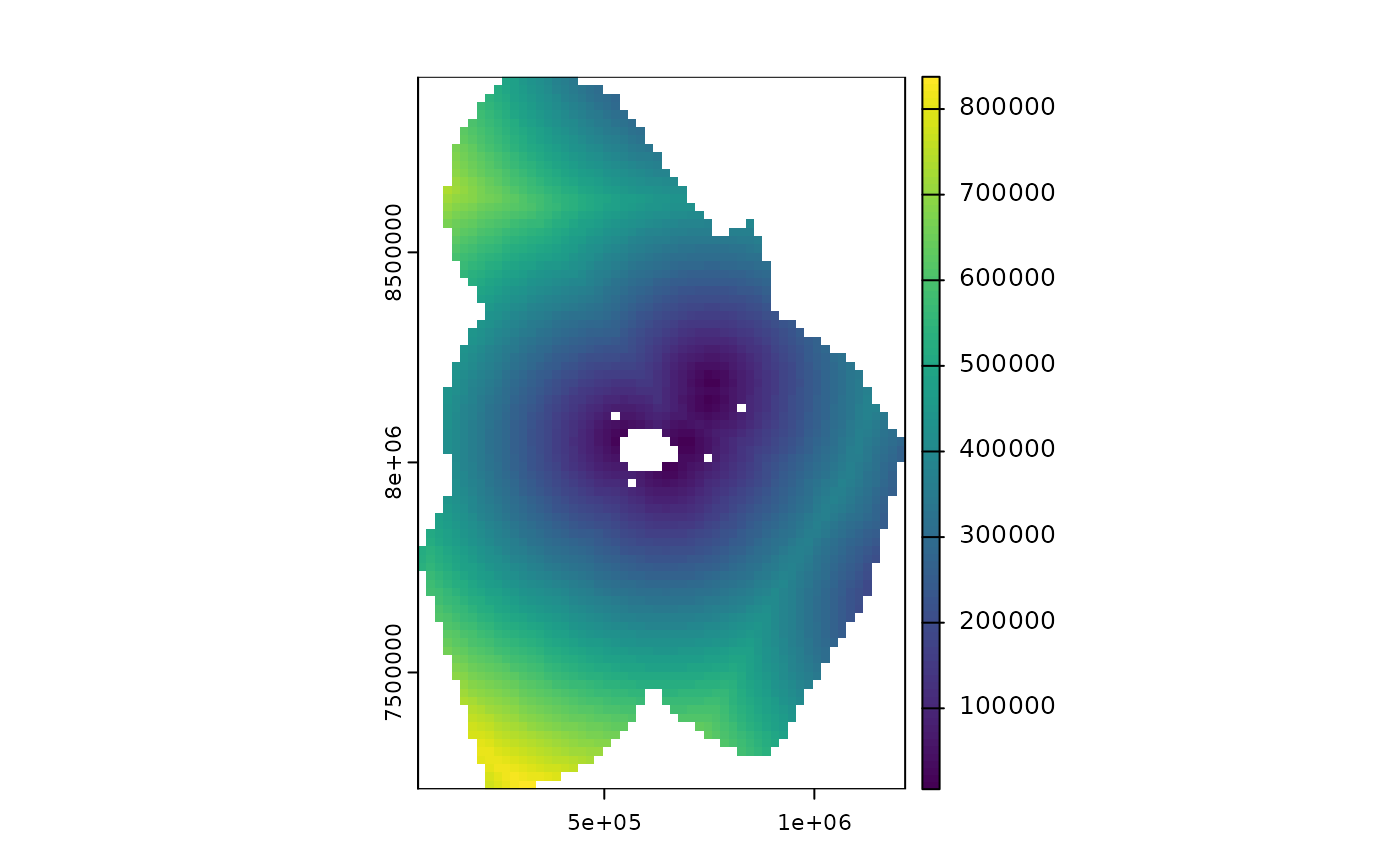#get distance to anchorages, as defined by Global Fishing Watch data
dist_anchorages <- get_dist(fiji_grid, dist_to = "anchorages_land_masked")
terra::plot(dist_anchorages)