Pacific High Seas Example • oceandatr

This example walks though how to do a spatial prioritization using oceandatr to obtain suitable data, and also using the package patchwise to ensure that entire seamounts are included in the prioritization solutions.

We use a High Seas area of the Pacific as the planning area for this example since it is outside any states’ jurisdiction.

#load oceandatr package
library(oceandatr)

Along with oceandatr we will need to load prioritizr for the spatial prioritization and we will use the open source solver lsymphony to solve the prioritization problem, so this needs to be installed and loaded via the Bioconductor website

library(gfwr)
library(prioritizr)
#remotes::install_bioc("lpsymphony")
library(lpsymphony)
#remotes::install_github("emlab-ucsb/patchwise")
library(patchwise)

High Seas area of the Pacific Ocean

First we retrieve geospatial data for the North Pacific Ocean using get_boundary(), then we will crop for the area we are interested in, the planning region, highlighted in red on the map.

high_seas <- get_boundary(type = "high_seas")

pacific_hs_area_extent <- sf::st_bbox(c(xmin = 135, xmax = 155, ymin = 0, ymax = 6), crs = 4326)

plot(sf::st_geometry(high_seas), main = "High Seas", col = "royalblue3", axes = TRUE, las = 1)
plot(pacific_hs_area_extent %>% sf::st_as_sfc() %>% sf::st_cast(to = "LINESTRING"), col = "red", lwd=2, add = TRUE)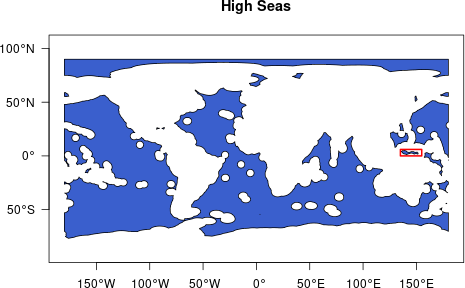

Map of the High Seas

We are going to use only the highlighted Pacific area which borders Indonesia, Papua New Guinea, Palau and the Federated States of Micronesia. We can get the EEZs of these states using oceandatr’s get_area function.


country_names <- c("Indonesia", "Papua New Guinea", "Palau", "Micronesia")

eezs <- lapply(country_names, FUN = function(x) get_boundary(name = x) %>% dplyr::select(territory1) %>% dplyr::rename(name = territory1)) %>% 
  do.call(rbind, .) %>% 
  sf::st_cast(to = "MULTIPOLYGON")

We only want the high seas portion of the area outlined above. We can create a polygon for this planning region by removing the bordering states EEZs.

sf::sf_use_s2(FALSE) #turn off S2 to avoid errors

pacific_hs <- high_seas %>%
  sf::st_crop(pacific_hs_area_extent) %>% 
  sf::st_sf() %>% 
  dplyr::mutate(name = "Planning region") %>% 
  dplyr::select(name)

sf::sf_use_s2(TRUE)

To make a nice context map, we can download bathymetry data using oceandatr’s get_bathymetry() function, using the bounding box of the EEZs as the input extent (grid). To get country boundaries to add to the map, we use the get_boundary() functions from oceandatr, setting name = NULL so that all countries are downloaded. We can then plot everything using the tmap package, which is great for making nice maps.


#retrieve bathymetry for the planning regions and surrounding area bounded by the EEZs
pacific_bathy <- get_bathymetry(spatial_grid = sf::st_as_sfc(sf::st_bbox(eezs), crs = 4326) %>% sf::st_as_sf(), raw = TRUE, classify_bathymetry = FALSE, resolution = 1) %>% 
  terra::classify(matrix(c(0, Inf, NA), ncol = 3))

#retrieve country boundaries using oceandatr
world <- get_boundary(name = NULL, type = "country")

tmap::tm_shape(pacific_bathy * -1) + #multiply bathymetry by -1 to make values positive for nicer legend
  tmap::tm_raster(
    col.scale = tmap::tm_scale_continuous(values = "brewer.yl_gn_bu"),
    col.legend = tmap::tm_legend(title = "Depth (m)", position = tmap::tm_pos_out("right"))
  ) +
  tmap::tm_shape(eezs %>% sf::st_cast(to = "MULTILINESTRING")) +
  tmap::tm_lines(
    col = "name",
    lwd = 1.5,
    col.scale = tmap::tm_scale_categorical(values = "brewer.dark2"),
    col.legend = tmap::tm_legend(title = "Select EEZs")
  ) +
  tmap::tm_shape(pacific_hs %>% sf::st_cast(to = "MULTILINESTRING")) +
  tmap::tm_lines(
    col = "name",
    lwd = 2,
    col.scale = tmap::tm_scale_categorical(values = "red"),
    col.legend = tmap::tm_legend(title = "")
  ) +
  tmap::tm_shape(world) +
  tmap::tm_borders() +
  tmap::tm_graticules(lwd = 0.5)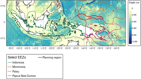

Map of Pacific High Seas planning region in regional context

Now we select a suitable projection for the area and a suitable resolution for the planning grid used for gridding the data. We can use projection wizard to find an equal-area projection, entering the same extent coordinates we used to crop the high seas area (xmin = 135, xmax = 155, ymin = 0, ymax = 6).

We will use 10km square planning units so that there the data processing and prioritization run reasonably fast (smaller planning units will require more time/ computer memory get data for)


pacific_hs_projection <- "+proj=cea +lon_0=145 +lat_ts=3 +datum=WGS84 +units=m +no_defs"

pacific_hs_planning_grid <- get_grid(boundary = pacific_hs,
                                     crs = pacific_hs_projection,
                                     resolution = 10000) 

#get_grid returns a raster by default, so we can plot it using the terra package. We convert it to polygons so we can see each grid square.
terra::plot(terra::as.polygons(pacific_hs_planning_grid, aggregate = FALSE))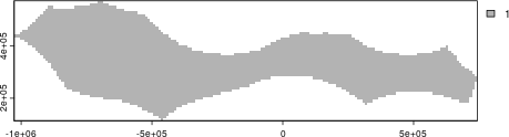

Pacific High Seas area planning grid raster

Now we have a planning grid, we can get data on conservation features (e.g. habitats) using oceandatr to use in a spatial prioritization with a single command get_features(). We have to set the seamount buffer, which is the area around the seamount that is included as part of the seamount, and we use 30km based since biodiversity is known to be higher within this distance of seamount peaks (see ?get_seamounts_buffered for more info).

#set seed for reproducibility in the get_enviro_zones() sampling to find optimal cluster number
set.seed(500)

feature_set <- get_features(spatial_grid = pacific_hs_planning_grid) %>% 
  remove_empty_layers()  #use this to remove raster layers that are empty

tmap::tm_shape(setNames(
  feature_set,
  gsub("_", " ", names(feature_set)) %>% stringr::str_to_sentence()
)) +
  tmap::tm_raster(
    col.scale = tmap::tm_scale_categorical(
      values = c("grey70", "royalblue"),
      labels = c("Absent", "Present")
    ),
    col.legend = tmap::tm_legend(show = FALSE)
  ) +
  tmap::tm_facets(ncol = 3) +
  tmap::tm_shape(pacific_hs %>% sf::st_transform(pacific_hs_projection)) +
  tmap::tm_borders() +
  tmap::tm_layout(panel.label.size = 1.5)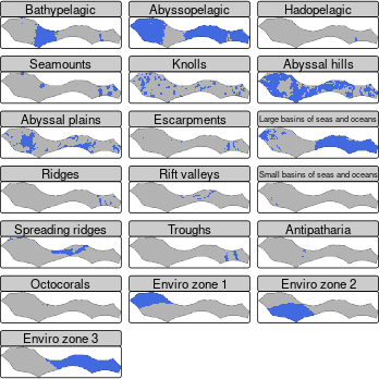

Map of all features in the planning regions

Cost data: Global Fishing Watch data

The other piece of data needed for a spatial prioritization is cost. In terrestrial spatial planning, this can be the actually monetary value of buying the land for conservation. In marine spatial planning, measures of fishing, such as catch and fishing effort, are often used as the opportunity cost for each planning unit.

Global Fishing Watch has global fishing effort data, and this can be accessed easily using get_gfw() function in oceandatr (which is a wrapper for the get_raster() function from the gfwr package). An API key is required, but can be easily generated at no cost; see the gfwr website for more details.


fishing_effort <- get_gfw(spatial_grid = pacific_hs_planning_grid, start_year = 2022, end_year = 2022, summarise = "total_annual_effort") %>% 
  terra::subst(NA, 0.01) %>% #set NA values to zero otherwise they will be left out of the prioritization
  terra::mask(pacific_hs_planning_grid) %>% 
  setNames("fishing_effort")

tmap::tm_shape(fishing_effort) +
  tmap::tm_raster(col.scale = tmap::tm_scale(values = "viridis"),
                  col.legend = tmap::tm_legend(orientation = "landscape",
                                               title = ""))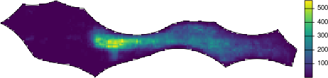

Map of total apparent fishing effort in 2022 for the Pacific High Seas area. Data from Global Fishing Watch

Run a simple spatial prioritization

We now have all the data we need to create a conservation problem and solve it to get a map of priority areas for conservation for our Pacific High Seas area. For the prioritization, we need to set targets for how much of each conservation feature must be included in the prioritized areas. We will set this at 20%.

prob <- prioritizr::problem(x = fishing_effort, features = feature_set) %>% 
  add_min_set_objective() %>% 
  add_relative_targets(0.2) %>% 
  #add_boundary_penalties(penalty = 0.00001) %>% 
  add_binary_decisions() %>% 
  add_lpsymphony_solver(verbose = FALSE)

sol <- solve(prob)

tmap::tm_shape(sol) +
  tmap::tm_raster(
    col.scale = tmap::tm_scale_categorical(values = c("grey70", "green4"),
                                           labels =  c("Not selected", "Selected")),
    col.legend = tmap::tm_legend(title = "",
                                 position = tmap::tm_pos_in("right", "top"))) +
  tmap::tm_shape(pacific_hs %>% sf::st_transform(pacific_hs_projection)) +
  tmap::tm_borders()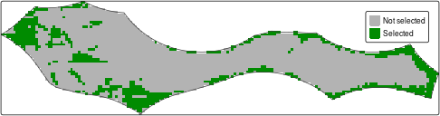

Prioritization solution for the Pacific High Seas area.

Prioritization with patches

Seamounts are known to be hotspots of biodiversity, so we might want to include only whole seamounts in the prioritization result, rather than parts of several seamounts. To ensure that whole seamount areas area included, we need to use the patchwise package to do some pre-processing of the data we use. The prioritization result is similar to that above, but whole seamount patches equal to at least 20% of the total seamount area are included.

# Separate seamount data - we want to protect entire patches
seamounts_rast <- feature_set[["seamounts"]]
features_rast <- feature_set[[names(feature_set)[names(feature_set) != "seamounts"]]]

# Create seamount patches - seamount areas that touch are considered the same patch
patches_rast <- patchwise::create_patches(seamounts_rast %>% terra::subst(0, NA)) #patchwise currently expects all non-patches to be NA, some subsituting non-seamounts, which are currently zeroes, with NAs

# Create patches dataframe - this creates several constraints so that entire seamount units are protected together
patches_df_rast <- patchwise::create_patch_df(spatial_grid = pacific_hs_planning_grid, features = features_rast, patches = patches_rast, costs = fishing_effort)
#> [1] "Processing patch 1 of 6"
#> [1] "Processing patch 2 of 6"
#> [1] "Processing patch 3 of 6"
#> [1] "Processing patch 4 of 6"
#> [1] "Processing patch 5 of 6"
#> [1] "Processing patch 6 of 6"

# Create boundary matrix for prioritizr
boundary_matrix_rast <- patchwise::create_boundary_matrix(spatial_grid = pacific_hs_planning_grid, patches = patches_rast, patch_df = patches_df_rast)

# Create targets for protection - let's just do 20% for each feature (including 20% of whole seamounts)
targets_rast <- patchwise::features_targets(targets = rep(0.2, (terra::nlyr(features_rast) + 1)), features = features_rast, pre_patches = seamounts_rast)

# Add these targets to targets for protection for the "constraints" we introduced to protect entire seamount units
constraints_rast <- patchwise::constraints_targets(feature_targets = targets_rast, patch_df = patches_df_rast)

# Run the prioritization
problem_rast <- prioritizr::problem(x = patches_df_rast, features = constraints_rast$feature, cost_column = "fishing_effort") %>%
  prioritizr::add_min_set_objective() %>%
  prioritizr::add_manual_targets(constraints_rast) %>%
  prioritizr::add_binary_decisions() %>%
  #prioritizr::add_boundary_penalties(penalty = 0.0001, data = boundary_matrix_rast) %>%
  prioritizr::add_lpsymphony_solver()

# Solve the prioritization
solution_rast <- solve(problem_rast)

# Convert the prioritization into a more digestible format
result_rast <- patchwise::convert_solution(solution = solution_rast, patch_df = patches_df_rast, spatial_grid = pacific_hs_planning_grid)

tmap::tm_shape(c(sol, result_rast)) +
  tmap::tm_raster(
    col.scale = tmap::tm_scale_categorical(values = c("grey70", "green4"),
                                           labels =  c("Not selected", "Selected")),
    col.legend = tmap::tm_legend(title = "",
                                 position = tmap::tm_pos_in("right", "top"))) +
  tmap::tm_shape(terra::as.polygons(seamounts_rast) |> sf::st_as_sf()) +
  tmap::tm_borders(col = "brown") +
  tmap::tm_shape(pacific_hs %>% sf::st_transform(pacific_hs_projection)) +
  tmap::tm_borders() +
  tmap::tm_layout(panel.labels = c("Original result", "Result with patchwise"))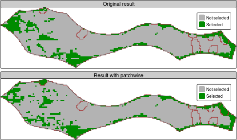

Prioritization solution for the Pacific High Seas area, with whole seamounts included. Brown outlines are seamounts.