Selecting areas with oceandatr
getarea_vignette.RmdThe get_area() function is used to generate an
sf object of the area of interest. If you already have an
sf object with your area of interest, you do not need to
use get_area() and can use your existing object in place of
an object returned by get_area(). However, if you do need
to generate an area of interest, using this particular function can be a
bit confusing if the desired area is not a well-defined EEZ. Here, we
walk through a few examples to make this function a little bit easier to
use and understand.
In the back-end, get_area() uses the
mrp_get() function from the mregions2
package - the R package for Marine Regions. This database is quite
extensive and has several options for querying areas. There are two
things to keep in mind when querying from this database - the query type
and the column of interest within that query.
We can get an idea of the possible query types using the following:
| title | layer |
|---|---|
| Exclusive Economic Zones (200 NM) (v11, world, 2019) | eez |
| Maritime Boundaries (v11, world, 2019) | eez_boundaries |
| Territorial Seas (12 NM) (v3, world, 2019) | eez_12nm |
| Contiguous Zones (24 NM) (v3, world, 2019) | eez_24nm |
| Internal Waters (v3, world, 2019) | eez_internal_waters |
| Archipelagic Waters (v3, world, 2019) | eez_archipelagic_waters |
| High Seas (v1, world, 2020) | high_seas |
| Extended Continental Shelves (v01, world, 2022) | ecs |
| Extended Continental Shelves - boundaries (v01, world, 2022) | ecs_boundaries |
| IHO Sea Areas (v3) | iho |
| Global Oceans and Seas (v1) | goas |
| The intersect of the Exclusive Economic Zones and IHO areas (v4) | eez_iho |
| Marine and land zones: the union of world country boundaries and EEZ’s | eez_land |
| Global Biogeochemical Provinces (Longhurst) | longhurst |
| Global contourite distribution | cds |
| Emission Control Areas (ECAs) designated under regulation 13 of MARPOL Annex VI (NOx emission control) | eca_reg13_nox |
| Emission Control Areas (ECAs) designated under regulation 14 of MARPOL Annex VI (SOx and particulate matter emission control) | eca_reg14_sox_pm |
| UNESCO World Heritage Marine Sites (v02, 2023) | worldheritagemarineprogramme |
| The 66 Large Marine Ecosystems of the World | lme |
| Marine Ecoregions of the World - Ecoregions | ecoregions |
| SeaVoX - Sea Areas Polygons (v18, 2021) | seavox_v18 |
There are several options to choose from, so it might be worthwhile
to do a little extra research to decide which layer is most likely to
give you the results you desire. Attributes in the “layer” column can be
used to inform the query_type in get_area().
From here, we can look at the list of possible column names to choose
from. Let’s use the “eez” option as the layer of interest and allow
show_column_options to equal TRUE.
get_area(query_type = "eez", show_column_options = TRUE)
#> $mregions_column
#>  [1] "mrgid"      "geoname"    "mrgid_ter1" "pol_type"   "mrgid_sov1" "territory1" "iso_ter1"   "sovereign1" "mrgid_ter2"
#> [10] "mrgid_sov2" "territory2" "iso_ter2"   "sovereign2" "mrgid_ter3" "mrgid_sov3" "territory3" "iso_ter3"   "sovereign3"
#> [19] "x_1"        "y_1"        "mrgid_eez"  "area_km2"   "iso_sov1"   "iso_sov2"   "iso_sov3"   "un_sov1"    "un_sov2"
#> [28] "un_sov3"    "un_ter1"    "un_ter2"    "un_ter3"
Each of these columns is a different type of identifier for ocean areas that we can choose from. A full explanation of what the columns mean can be found here. The column we choose depends on how we want to refer to the area that we choose. Perhaps the most common column we might use is “territory1”, which allows us to provide a specific country name by which to query. For example, we can pull Australia’s EEZ and plot the result:
# Grab the area
australia_eez <- get_area(area_name = "Australia", query_type = "eez", mregions_column = "territory1")

# Plot the result
plot(australia_eez[2])
Map of the Australian EEZ.
Alternatively, we might know the ISO3 code for a territory and wish to query the database that way; we would use the “iso_ter1” column to filter for the ISO3 code we desire. Below, we use the ISO3 code for Australia to grab the EEZ.
# Grab the area
australia_eez <- get_area(area_name = "AUS", query_type = "eez", mregions_column = "iso_ter1")

# Plot the result
plot(australia_eez[2])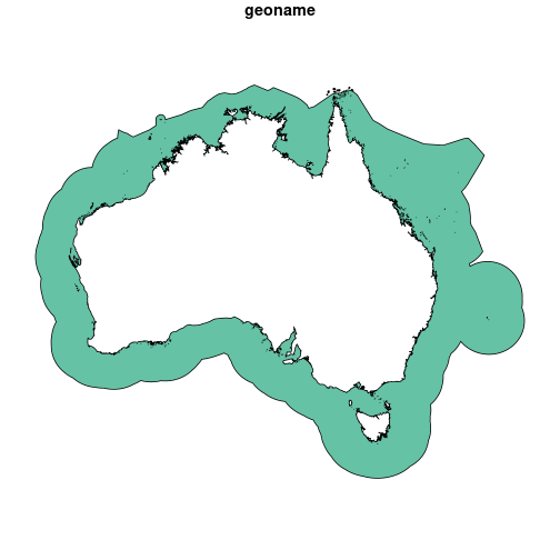
Map of the Australian EEZ.
Of course, maybe we aren’t memorizing ISO3 codes, but we would
recognize the code that we wanted if we saw it in a list. We can get a
list of possible values to choose from for each
mregions_column by setting show_value_options
to TRUE:
get_area(query_type = "eez", mregions_column = "iso_ter1", show_value_options =  TRUE)
#> $iso_ter1
#>   [1] "ABW" "AGO" "AIA" "ALB" "ARE" "ARG" "ASM" "ATF" "ATG" "AUS" "AZE" "BEL" "BEN" "BES" "BGD" "BGR" "BHR" "BHS" "BIH"
#>  [20] "BLM" "BLZ" "BMU" "BRA" "BRB" "BRN" "CAN" "CCK" "CHL" "CHN" "CIV" "CMR" "COD" "COG" "COK" "COL" "COM" "CPV" "CRI"
#>  [39] "CUB" "CUW" "CXR" "CYM" "CYP" "DEU" "DJI" "DMA" "DNK" "DOM" "DZA" "ECU" "EGY" "ERI" "ESH" "ESP" "EST" "FIN" "FJI"
#>  [58] "FLK" "FRA" "FRO" "FSM" "GAB" "GBR" "GEO" "GGY" "GHA" "GIB" "GIN" "GLP" "GMB" "GNB" "GNQ" "GRC" "GRD" "GRL" "GTM"
#>  [77] "GUF" "GUM" "GUY" "HMD" "HND" "HRV" "HTI" "IDN" "IMN" "IND" "IRL" "IRN" "IRQ" "ISL" "ISR" "ITA" "JAM" "JEY" "JOR"
#>  [96] "JPN" "KAZ" "KEN" "KHM" "KIR" "KNA" "KOR" "KWT" "LBN" "LBR" "LBY" "LCA" "LKA" "LTU" "LVA" "MAF" "MAR" "MCO" "MDG"
#> [115] "MDV" "MEX" "MHL" "MLT" "MMR" "MNE" "MNP" "MOZ" "MRT" "MSR" "MTQ" "MUS" "MYS" "MYT" "NAM" "NCL" "NFK" "NGA" "NIC"
#> [134] "NIU" "NLD" "NOR" "NRU" "NZL" "OMN" "PAK" "PAN" "PCN" "PER" "PHL" "PLW" "PNG" "POL" "PRI" "PRK" "PRT" "PSE" "PYF"
#> [153] "QAT" "REU" "ROU" "RUS" "SAU" "SDN" "SEN" "SGP" "SGS" "SHN" "SJM" "SLB" "SLE" "SLV" "SOM" "SPM" "STP" "SUR" "SVN"
#> [172] "SWE" "SXM" "SYC" "SYR" "TCA" "TGO" "THA" "TKL" "TKM" "TLS" "TON" "TTO" "TUN" "TUR" "TUV" "TWN" "TZA" "UKR" "UMI"
#> [191] "URY" "USA" "VCT" "VEN" "VGB" "VIR" "VNM" "VUT" "WLF" "WSM" "YEM" "ZAF"
There might be a project in which you need the area in the high seas.
This is a little tricky, but easy if you know the codes. In this case,
the area_name should be “63202”, the
query_type should be “high_seas”, and the
mregions_column should be “mrgid”. There is only one option
for the high seas area, and it returns the layer in its entirety.
# Grab the area
high_seas <- get_area(area_name = "63203", query_type = "high_seas", mregions_column = "mrgid")

# Plot the result
plot(high_seas[2])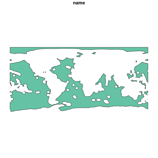
Map of the high seas.
If you are only interested in a small section of the high seas, you can crop this layer to the appropriate extent.
sf::sf_use_s2(FALSE) # turn of spherical geometry so we can crop

# Crop the area
high_seas_cropped <- high_seas %>%
  sf::st_crop(xmin = 100, xmax = 185, ymin = -60, ymax = 0)

# Plot the result
plot(high_seas_cropped[2])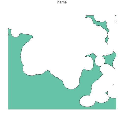
Map of the high seas, cropped near Australia.
If your region of interest includes the high seas and an EEZ area,
you can combine the two layers resulting from their independent queries
using sf::st_union().
# Combine the areas
australia_eez_high_seas <- australia_eez %>%
  sf::st_union(high_seas_cropped)

# Plot the result
plot(australia_eez_high_seas[2])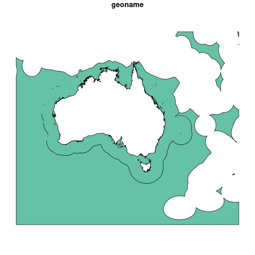
Map of the Australian EEZ and nearby high seas areas.
Currently, there is no way to select multiple areas at once. If your region of interest spans several EEZs or marine regions, we recommend querying each area independently and merging the layers together.
# Grab the area
indonesia_eez <- get_area(area_name = "Indonesia", query_type = "eez", mregions_column = "territory1")

# Combine the areas
australia_indonesia <- australia_eez %>%
  sf::st_union(indonesia_eez)

# Plot the result
plot(australia_indonesia[2]) 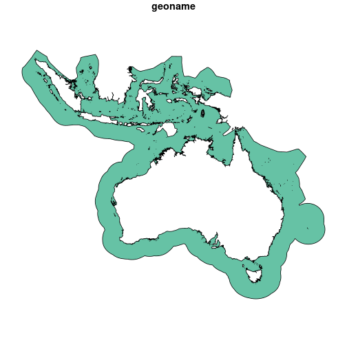
Map of the Indonesian and Australian EEZs.
We can now go ahead and use these areas in oceandatr to
create an appropriate planning grid and grab additional datasets.
# Set projection for planning grid - grabbed from this website: https://projectionwizard.org
projection <- 'PROJCS["ProjWiz_Custom_Albers",
 GEOGCS["GCS_WGS_1984",
  DATUM["D_WGS_1984",
   SPHEROID["WGS_1984",6378137.0,298.257223563]],
  PRIMEM["Greenwich",0.0],
  UNIT["Degree",0.0174532925199433]],
 PROJECTION["Albers"],
 PARAMETER["False_Easting",0.0],
 PARAMETER["False_Northing",0.0],
 PARAMETER["Central_Meridian",135],
 PARAMETER["Standard_Parallel_1",-45.850866],
 PARAMETER["Standard_Parallel_2",3.0571749],
 PARAMETER["Latitude_Of_Origin",-21.3968456],
 UNIT["Meter",1.0]]'

# Create a planning grid
planning_grid <- get_grid(area_polygon = australia_indonesia,
                                   projection_crs = projection,
                                   resolution = 10000)

# Plot the planning grid
terra::plot(planning_grid, box = FALSE, axes = FALSE, legend = FALSE)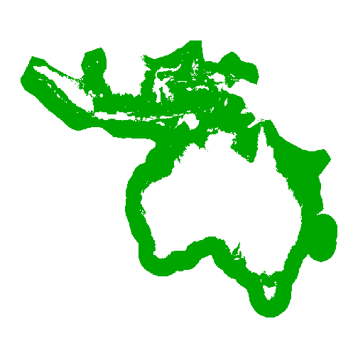
Planning grid of the Indonesian and Australian EEZs.
# Get seamount locations with a 30 km buffer
seamounts <- get_seamounts_buffered(spatial_grid = planning_grid,
                                    buffer = 30000)
# Plot seamount data
terra::plot(seamounts, box = FALSE, axes = FALSE, legend = FALSE)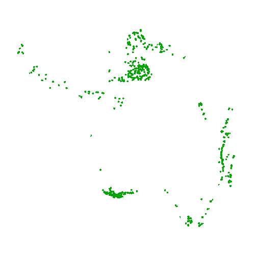
Seamounts within the Indonesian and Australian EEZs.