2 Dark fleet emissions model
The dark emissions model uses Sentinel-1 (S1) Synthetic Aperture Radar (SAR) data to estimate emissions from the ‘dark fleet’—vessels that do not broadcast AIS and are therefore not captured in AIS-based datasets (Rowlands et al. (2019)).
2.1 Methods
2.1.1 Model overview
To estimate emissions from the dark fleet, we spatiotemporally extrapolate our AIS-based emissions estimates to the dark fleet based on spatiotemporal vessel detections. For every S1 detection, GFW has determined whether or not the vessel is matched to an AIS vessel that was broadcasting at the same location and time, allowing us to determine the number of AIS-broadcasting and dark vessels in a given location and time. We can also make this extrapolation disaggregated by vessel type and length, as the GFW S1 model can identify whether each dark fleet detection represents a fishing or non-fishing vessel and determine its length. See Paolo et al. (2024) for further information on the S1 detection model.
Our approach for estimating emissions for the dark fleet is as follows:
- Grid the ocean to 1x1 degree pixels.
- Use a monthly temporal aggregation unit.
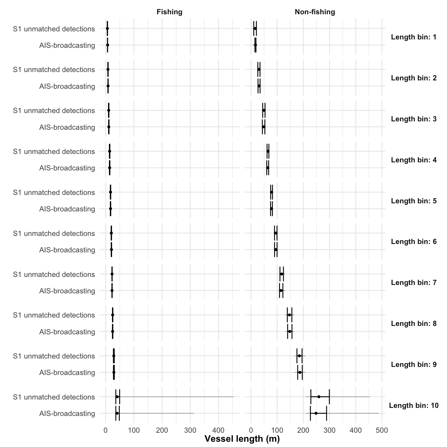
- For each vessel type (fishing and non-fishing), use length percentiles to bin vessels into one of the 10 size classes. We set the bins from the S1 unmatched detected lengths and apply the same cutoffs to both the AIS-based vessel characteristics and the S1-detected vessel lengths. We then extrapolate AIS-based emissions to dark emissions within each size class, mapping generally larger AIS-broadcasting vessels to generally larger dark vessels and smaller to smaller. Looking at Figure 2.1, the size distributions for fishing vessels across the length bins are very similar between S1 unmatched detections and AIS-broadcasting vessels. We use 10 bins based on a sensitivity analysis, beyond which total emissions stabilize. Discrete size classes (rather than a continuous length relationship) let each class carry the aggregated trip characteristics embedded in the AIS gridded emissions—such as time and distance traveled within a pixel—which cannot be inferred from S1 imagery alone.
For each 1x1 degree pixel, month, vessel type (fishing or non-fishing), and vessel size class, use our AIS-based emissions model to determine the amount of AIS-based emissions for each of the nine pollutants (CO2, CH4, N2O, NOX, SOX, CO, PM2.5, PM10, and VOCs)
For each 1x1 degree pixel, month, vessel type, and vessel size class, use S1 SAR data to determine the following: 1) the number vessel detections that are matched to an AIS-broadcasting vessel; 2) the number vessel detections that are not matched to an AIS-broadcasting vessel (i.e., the number of dark vessels); and 3) the ratio of dark vessels to AIS-broadcasting vessels.
Assigning missing ratios: S1 does not provide complete global spatial coverage—its footprint is set by the satellite’s orbital path and the presence of land, leaving most of the open ocean and some coastal areas unobserved. We fill in missing ratios using K-nearest neighbors (KNN), averaging the ratios of the 8 closest pixels that have a value, separately by month, vessel type, and vessel size class. We do this in two cases: for pixels inside the footprint that have detections but no AIS match (
NULLratios), and for pixels outside the footprint entirely. For pixels outside the footprint, we additionally smooth the KNN ratios across neighboring pixels. We use k = 8 based on a sensitivity analysis (it maximizesrsq_tradwhen inferring ratios for pixels with known values). Neighbor selection is exact and global: we precompute center-to-center spheroid distances between every pair of pixels on a fixed global ocean grid, and select each pixel’s 8 nearest neighbors with known ratios from that table with no distance cutoff. (Earlier model versions restricted the neighbor search to within 25 degrees latitude and longitude for computational tractability, which silently left remote open-ocean pixels—roughly 11% of ocean pixels in a typical month—without assigned ratios; this restriction was removed in the July 2026 model version.)Using these ratios, we multiply our AIS-based emissions estimates by the ratio of dark vessels to AIS-broadcasting vessels, for each pollutant by pixel, month, and vessel category. We use the pixel-level monthly ratio where available, then the within-footprint KNN ratio for null pixels inside the footprint, and finally the outside-footprint KNN ratio for pixels beyond S1 coverage.
This then gives us, for every month and location where AIS-based emissions estimates are available, corresponding dark fleet emissions estimates. Adding these two numbers together gives us yearly gridded total emissions estimates from across the AIS-broadcasting and dark fleets.
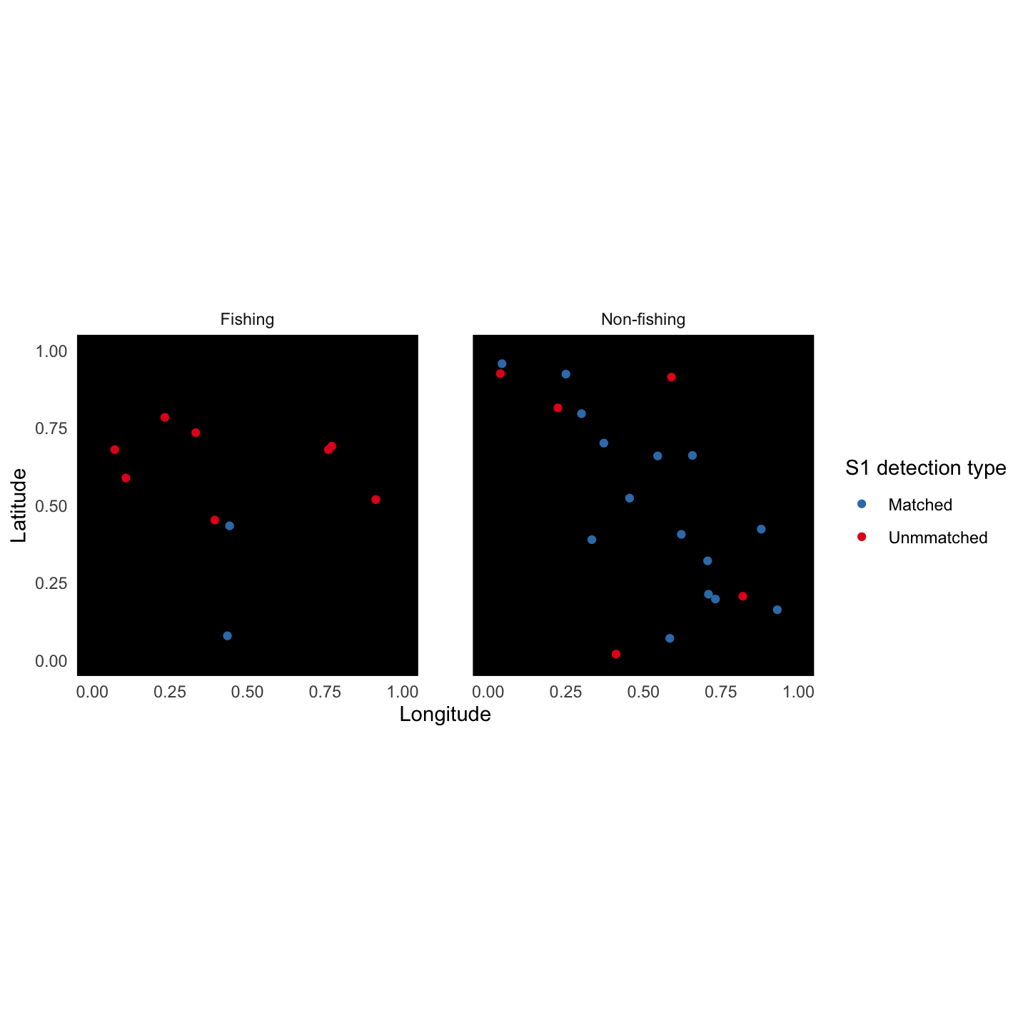
As an example, we can look at a hypothetical 1x1 degree pixel, in a hypothetical month, representing the S1 detections corresponding to a specific vessel size bin (Figure 2). We can see detections for fishing vessels and non-fishing vessels (e.g., cargos, tankers, etc). First, we consider fishing vessels. Here we can see that S1 had 2 detections that we were able to match to AIS-broadcasting vessels, and 8 detections which were unmatched (e.g., these are from dark vessels). Therefore, the ratio of dark-to-AIS-broadcasting vessels is 8/2 = 4. For this pixel, month, vessel type, and size bin, we would therefore take our AIS-broadcasting emissions and multiply it by 4 to obtain our dark emissions estimate. If our observed AIS-broadcasting emissions for fishing vessels was 5 metric tonnes of CO2, our dark emissions would be 5*4 = 20 metric tonnes of CO2. This calculation is done for each of the nine pollutants.
Next, we consider non-fishing vessels. Here we can see that S1 had 15 detections that we were able to match to AIS-broadcasting vessels, and 5 detections which were unmatched (e.g., these are from dark vessels). Therefore, the ratio of dark-to-AIS-broadcasting vessels is 5/15 = 0.33. For this pixel, month, size bin, we would therefore take our AIS-broadcasting emissions and multiply it by 0.33 to obtain our dark emissions estimate. If our observed AIS-broadcasting emissions were 60 metric tonnes of CO2 for non-fishing vessels, our dark emissions would be 60*0.33 = 20 metric tonnes of CO2. This calculation is done for each of the nine pollutants.
2.1.2 Data
2.1.2.1 S1 vessel detections
The S1 vessel detections table includes all the necessary variables to determine detection locations, timestamps, lengths and whether each detection is matched to an AIS-broadcasting vessel. It also contains the required parameters for filtering out noise. We use the sentinel1_clean_v20250827 detection table.
Below is a summary of the variables included:
detect_id: Unique S1 vessel detection id.corrected_length_m: Inferred length from S1 detection, which has additionally been corrected for small vessels <22m using the relationship between known length and inferred length based on years of confident matches.presence: Presence of a vessel in the S1 detection. A value >0.7 indicates the reliable presence of a vessel.ssvid: ssvid (MMSI for AIS) of any AIS-broadcasting vessel spatiotemporally matched to the S1 detection.detect_lat: Latitude of vessel detection.detect_lon: Longitude of vessel detection.detect_timestamp: Timestamp of vessel detectionmatching_score: Score for determining whether the S1 detection is matched to an AIS-broadcasting vessel. When(matching_score > 4.22E-5 OR IFNULL(matching_score_secondary, 0) > 0.05) AND valid_segment, we classify the detection as matched to an AIS-broadcasting vessel. The secondary matching score recovers matches that the primary score misses.confidence: Confidence in the match between the S1 detection and any AIS vessel, indicating the level of ambiguity in the match. If there are multiple detections and AIS vessels very close to each other, the matching score of each possible pair would be similar and the confidence would be low. In contrast, if there’s only one possible pair, the confidence would be high no matter what the score is. In cases where there are multiple potentialssvidmatches for a singledetect_id, we select the match with the highest confidence.repeated_detections: Flags repeated S1 detections that may represent fixed infrastructure rather than actual vessels (objects recurring in nearly the same location over time). We exclude these detections.at_known_anchorages: Vessels in anchorages are excluded to receive the same treatment as those within the 1nm coastal buffer, for which S1 currently lacks the capacity to properly classify as vessels. Although there is potential for improvement, as discussed and tested in GitHub issue #11, the impact on overall emissions is minimal.- Additional filtering is applied to reduce noise and exclude detected objects that may not be vessels, using the variables
likely_ambiguities,likely_infrastructure,likely_vehicles_on_roads, andpotential_ice.
2.1.2.2 S1 classification of whether each detection is fishing or not
To determine whether each S1 vessel detection is a fishing vessel, we use GFW’s model, which classifies each detection and defines its likelihood of being a fishing vessel (Paolo et al. (2024)). The variables of interest from these tables pipe_sar_v1_published.fishing_pred_even_cal and pipe_sar_v1_published.fishing_pred_odd_cal are:
detect_id: Unique S1 vessel detection id.fishing_50: Fishing score of the vessel. If this value is > 0.5, then we classify the vessel type as fishing. Otherwise, we classify the vessel type as non-fishing.
2.1.3 Areas of potential model refinement
We have identified several areas for potential model refinement:
Ratios outside the footprint: The KNN approach outperforms global ratios, but assigning ratios beyond the S1 footprint remains the largest source of uncertainty. Two artifacts stand out. First, sharp changes can appear at the footprint boundary: pixels just outside the footprint draw on farther, denser coastal neighbors, which can inflate their ratios relative to adjacent pixels inside the footprint and overestimate open-ocean emissions. Second, vessel groups that are unevenly detected within the footprint (e.g., large non-fishing vessels) can propagate concentrated, high-contrast ratio patches into the open ocean, an effect that is more pronounced at the monthly level. We apply focal smoothing to the KNN ratios to reduce the most evident anomalies, but this remains the area with the greatest room for improvement. More sophisticated extrapolation—such as Kriging or machine learning—could assign ratios using not only spatial proximity but also temporal proximity, ocean basin, vessel characteristics, distance to shore and ports, and traffic routes.
Model performance: No comprehensive dataset exists for validating dark fleet emissions directly. We therefore do not have a robust way of validating our dark fleet emissions.
Sentinel-2 data: We use S1 SAR data for our estimates. Sentinel-2 (S2) optical imagery could extend coverage, but differences in detection capacity, coverage, and noise prevent integrating it directly with S1. Combining the two datasets is a target for future work.
2.2 Results
Dark emissions for CO2 accounted for 25% of total emissions in 2025. The following sections explore these results in more detail, including resolution by vessel category and spatial variability.
2.2.1 Ratio of the dark fleet to the AIS-broadcasting fleet
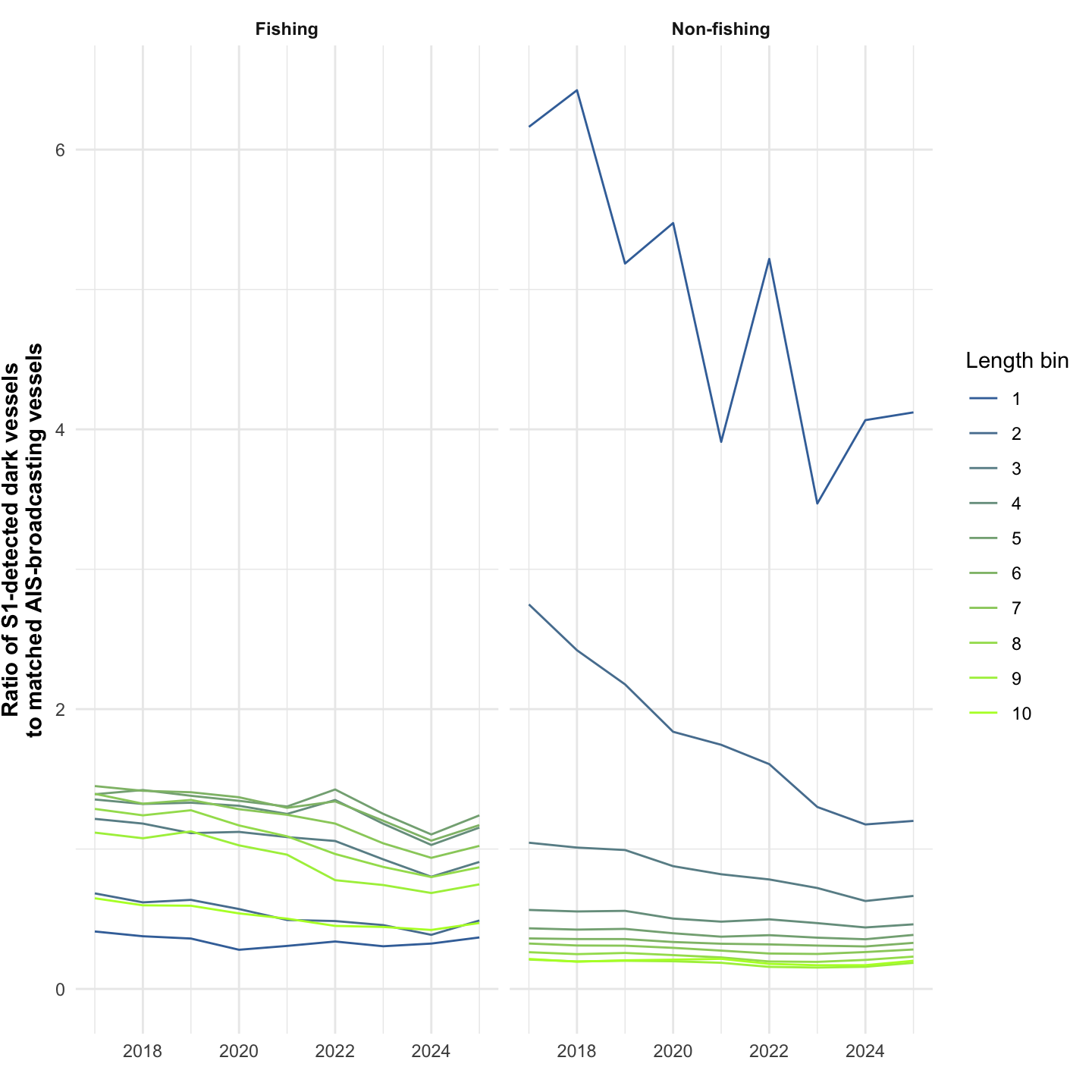
First, we visualize the ratio of the dark fleet to the AIS-broadcasting fleet observed within the S1 spatiotemporal footprint (Figure 2.3). This ratio serves as the basis for extrapolating AIS-based emissions to dark fleet emissions. We can look at how the ratio changes over years, disaggregated by vessel type and size class. For each year, vessel type, and size class, this ratio represents the aggregate month ratio within the S1 spatial footprint (i.e., the total number of unmatched dark vessel detections to the total number of matched AIS-broadcasting detections). Matching intuition, fishing vessels tend to have a higher ratio of dark-to-AIS vessels than non-fishing vessels, and smaller vessels tend to have a higher ratio than larger vessels (Table 2.1). Also matching intuition, the ratio of dark-to-AIS vessels is generally decreasing over time as more vessels use AIS and AIS coverage improves.
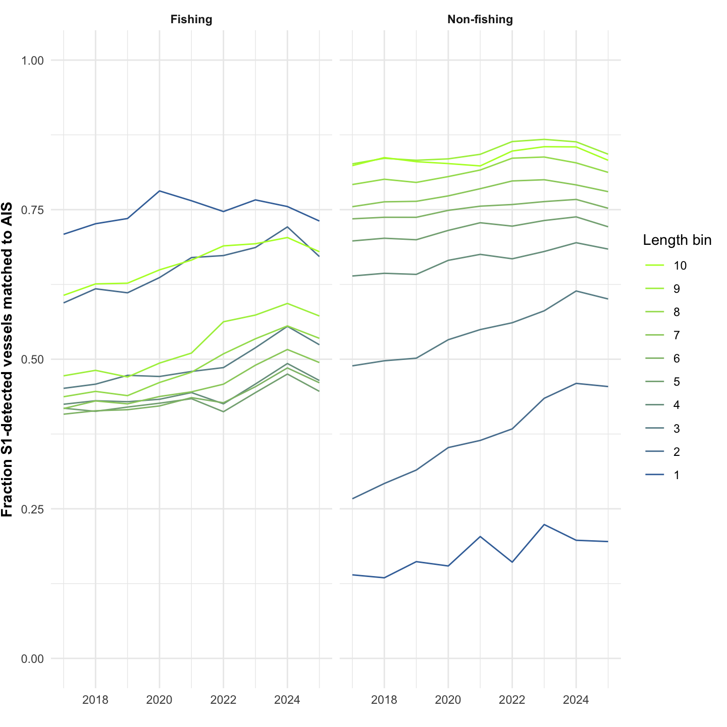
Another way to visualize these data is to look at the fraction of all detected vessels that are matched to AIS (i.e., the number of AIS-broadcasting detections divided by the total number of detections across the AIS-broadcast and dark fleets) (Figure 2.4). This is the metric reported by Paolo et al. (2024). Matching intuition, non-fishing vessels tend to have a higher fraction of S1 detections matched to AIS than fishing vessels, and larger vessels tend to have a higher fraction of detections matched to AIS than smaller vessels (Table 2.1). While the relative patterns align—non-fishing vessels are tracked at higher rates than fishing vessels—our estimates are higher compared to those of Paolo et al. (2024), who analyzed data from 2017-2021 and estimated that 70-79% of non-fishing vessels and 24-28% of fishing vessels are tracked with AIS.
| fleet | ratio_dark_to_ais_detections | fraction_tracked |
|---|---|---|
| Fishing | 0.934 | 0.517 |
| Non-fishing | 0.339 | 0.747 |
2.2.2 Emissions
Next, we look at the total annual global emissions for each of our pollutants over time (see Figure 2.5, Table 2.2), disaggregated by the AIS-broadcasting fleet and the dark fleet as detected by S1.
To summarize some additional key findings:
Industrial vessels emitted approximately 1.6 billion tons of CO2 in 2025, accounting for about 4.2% of global fossil fuel emissions ((IEA) (2023)).
Maritime emissions are likely growing at more than twice the rate of global CO2 emissions. Between 2017 and 2025, global fossil fuel emissions increased by 7% ((IEA) (2023)), while emissions from maritime vessels grew by 33%.
While 15% of maritime emissions in 2025 came from ‘high-information’ vessels that broadcast their positions via AIS and have IMO numbers, 60% came from ‘low-information’ AIS-broadcasting vessels without IMO numbers, and 25% came from dark fleet vessels that do not broadcast AIS. Understanding low-information and dark fleet activity is crucial for estimating total emissions and tracking changes over time. Emissions from dark vessels decreased by 9% between 2017 and 2025, whereas emissions from AIS-broadcasting vessels rose by 44% over the same time period. This shift is largely due to increased AIS adoption and advancements in AIS technology.
Our analysis also revealed seasonal and event-driven variations in emissions. Emissions consistently dipped during major holidays, including Christmas, New Year’s Day, and Chinese New Year, and also fell during the COVID-19 pandemic. Furthermore, our analysis also shows changes in the geographical distribution of emissions that are likely driven by new policies and infrastructure development.
Our AIS-based emissions estimates align closely with other published sources: the latest EDGAR estimates from 2024 are 860 MMT; the latest OECD estimates from 2024 are 862 MMT; the latest IMO estimates from 2018 are 1.06 B MT; and we estimate approximately 1.5 B MT CO2 in 2024.
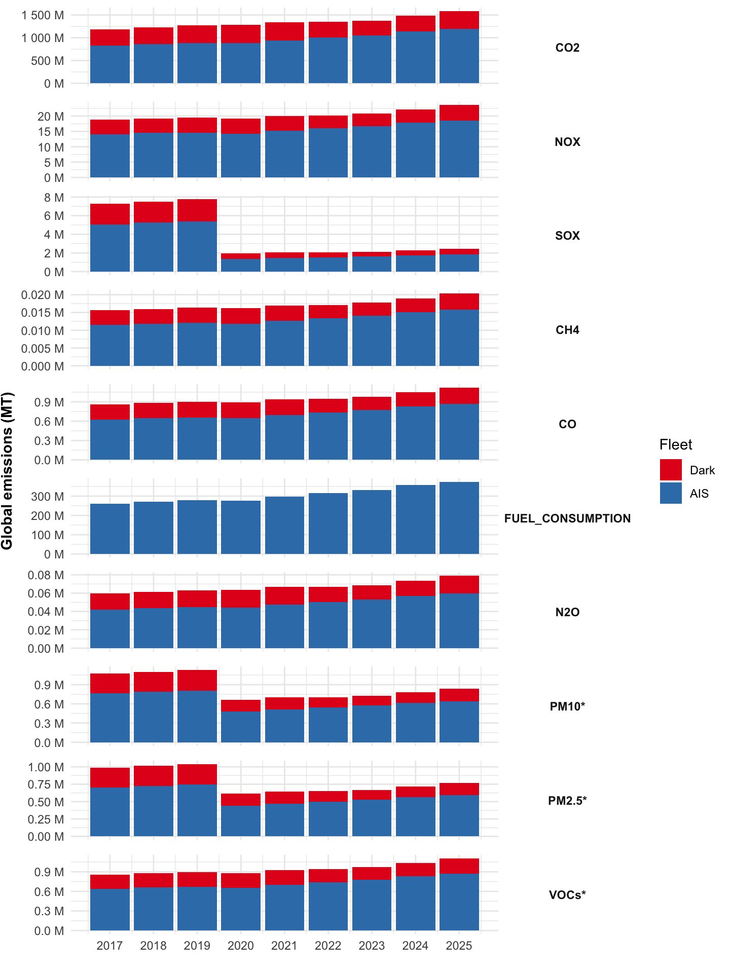
| year | Fleet | CO2 | NOX | SOX | CH4 | CO | N2O | PM10 | PM2_5 | VOCS | FUEL_CONSUMPTION |
|---|---|---|---|---|---|---|---|---|---|---|---|
| 2017 | Dark | 364,562,636 | 4,698,819 | 2,249,855 | 4,146 | 232,011 | 17,779 | 308,759 | 284,057 | 215,639 | NA |
| 2018 | Dark | 367,487,679 | 4,677,139 | 2,268,136 | 4,145 | 232,237 | 17,893 | 310,249 | 285,454 | 215,329 | NA |
| 2019 | Dark | 383,013,802 | 4,832,674 | 2,360,853 | 4,296 | 240,697 | 18,618 | 322,277 | 296,534 | 223,795 | NA |
| 2020 | Dark | 404,097,021 | 4,864,227 | 622,013 | 4,340 | 245,085 | 19,536 | 185,386 | 170,554 | 225,574 | NA |
| 2021 | Dark | 403,137,472 | 4,852,577 | 620,423 | 4,328 | 244,245 | 19,483 | 184,932 | 170,142 | 225,325 | NA |
| 2022 | Dark | 340,536,428 | 4,197,183 | 525,142 | 3,766 | 211,518 | 16,498 | 159,434 | 146,680 | 196,588 | NA |
| 2023 | Dark | 314,402,041 | 4,092,491 | 484,806 | 3,691 | 205,317 | 15,357 | 153,256 | 141,014 | 192,485 | NA |
| 2024 | Dark | 341,609,976 | 4,275,709 | 527,078 | 3,870 | 216,508 | 16,594 | 162,514 | 149,521 | 201,426 | NA |
| 2025 | Dark | 397,161,771 | 5,082,072 | 612,987 | 4,601 | 256,374 | 19,361 | 191,915 | 176,578 | 240,632 | NA |
| 2017 | AIS | 824,218,655 | 14,107,633 | 5,025,029 | 11,473 | 627,651 | 41,785 | 761,982 | 701,023 | 640,725 | 259,665,170 |
| 2018 | AIS | 861,417,974 | 14,503,805 | 5,247,862 | 11,845 | 648,872 | 43,550 | 791,224 | 727,926 | 660,289 | 271,384,574 |
| 2019 | AIS | 884,081,785 | 14,601,273 | 5,389,357 | 12,030 | 659,256 | 44,566 | 807,368 | 742,779 | 668,481 | 278,524,749 |
| 2020 | AIS | 879,054,702 | 14,277,525 | 1,344,155 | 11,823 | 648,498 | 44,247 | 480,261 | 441,841 | 655,818 | 276,941,106 |
| 2021 | AIS | 941,098,607 | 15,219,708 | 1,440,008 | 12,594 | 691,790 | 47,391 | 513,630 | 472,539 | 699,712 | 296,487,859 |
| 2022 | AIS | 1,004,524,398 | 16,021,251 | 1,539,676 | 13,383 | 735,331 | 50,428 | 545,481 | 501,843 | 742,249 | 316,470,057 |
| 2023 | AIS | 1,054,249,167 | 16,739,653 | 1,617,398 | 14,150 | 775,723 | 52,905 | 573,653 | 527,761 | 781,788 | 332,135,589 |
| 2024 | AIS | 1,139,197,974 | 17,866,397 | 1,749,804 | 15,131 | 830,746 | 57,062 | 615,808 | 566,544 | 834,948 | 358,898,539 |
| 2025 | AIS | 1,189,412,753 | 18,473,718 | 1,829,501 | 15,760 | 864,984 | 59,523 | 640,958 | 589,681 | 867,643 | 374,718,694 |
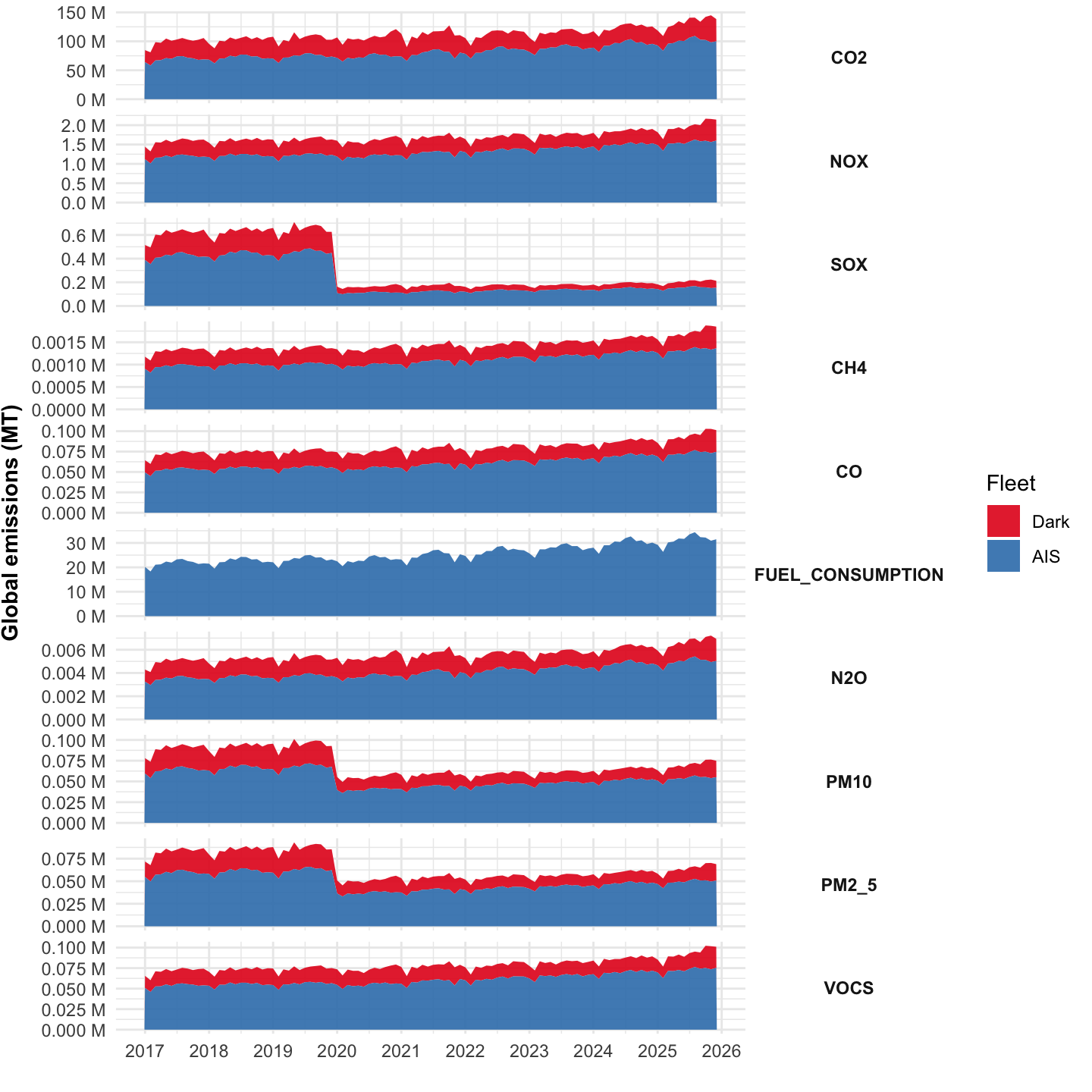
The same results, disaggregated by month, show a similar trend with total emissions increasing over the years (see Figure 2.6).
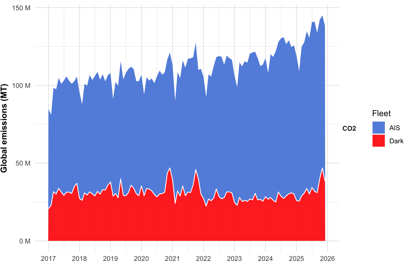
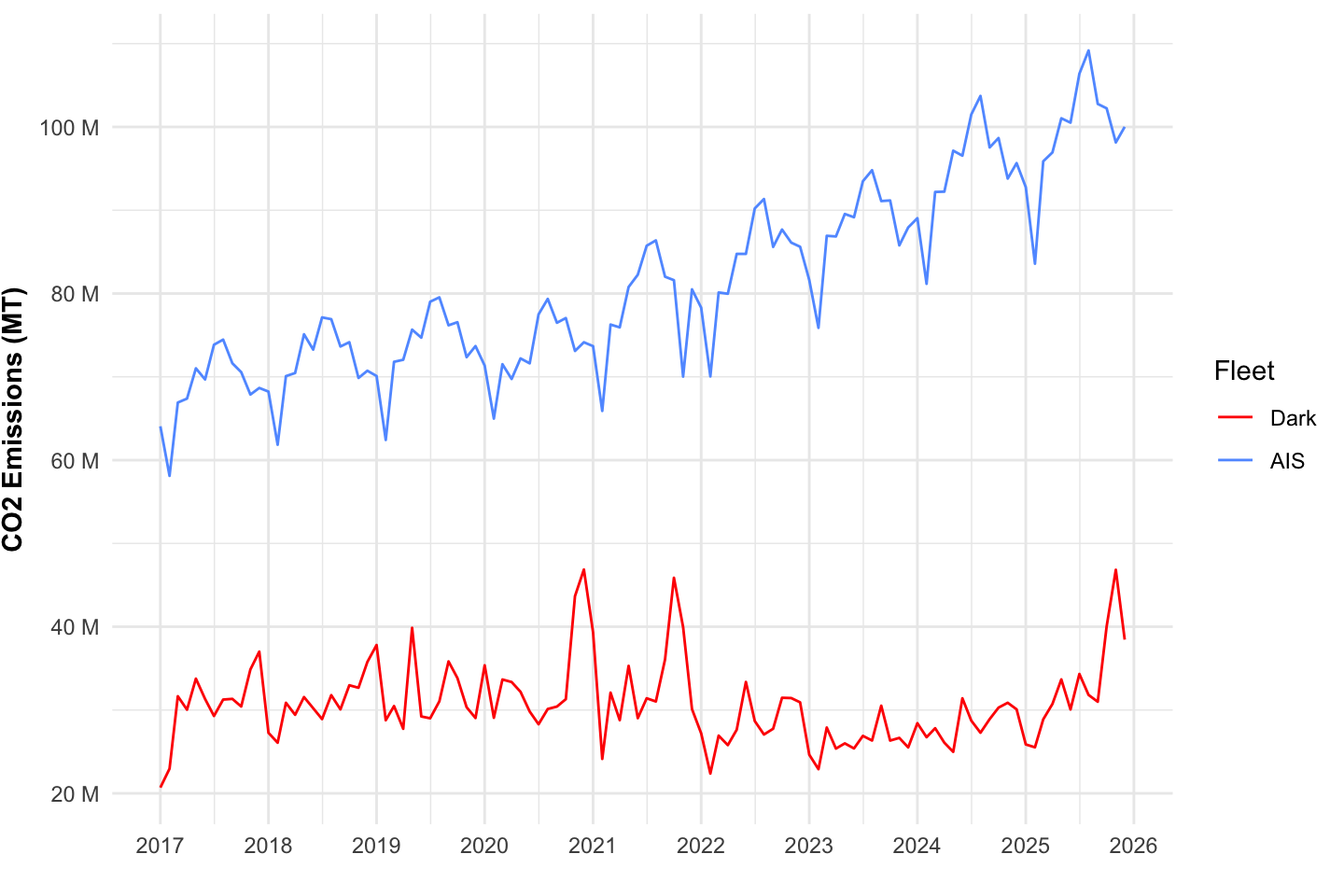
Displaying a single pollutant, such as CO2 (see Figure 2.7), we can clearly see an increase in total emissions over the years, and certain seasonality in the total emissions. Furthermore, Figure 2.7 and Figure 2.8 clearly depict the increase in AIS emissions versus a slight decrease in dark emissions, potentially linked to an improved in AIS coverage over the years. Despite dark emissions being derived from AIS emissions, the model also captures independent temporal variability in dark emissions, as evidenced by distinct seasonal trends.
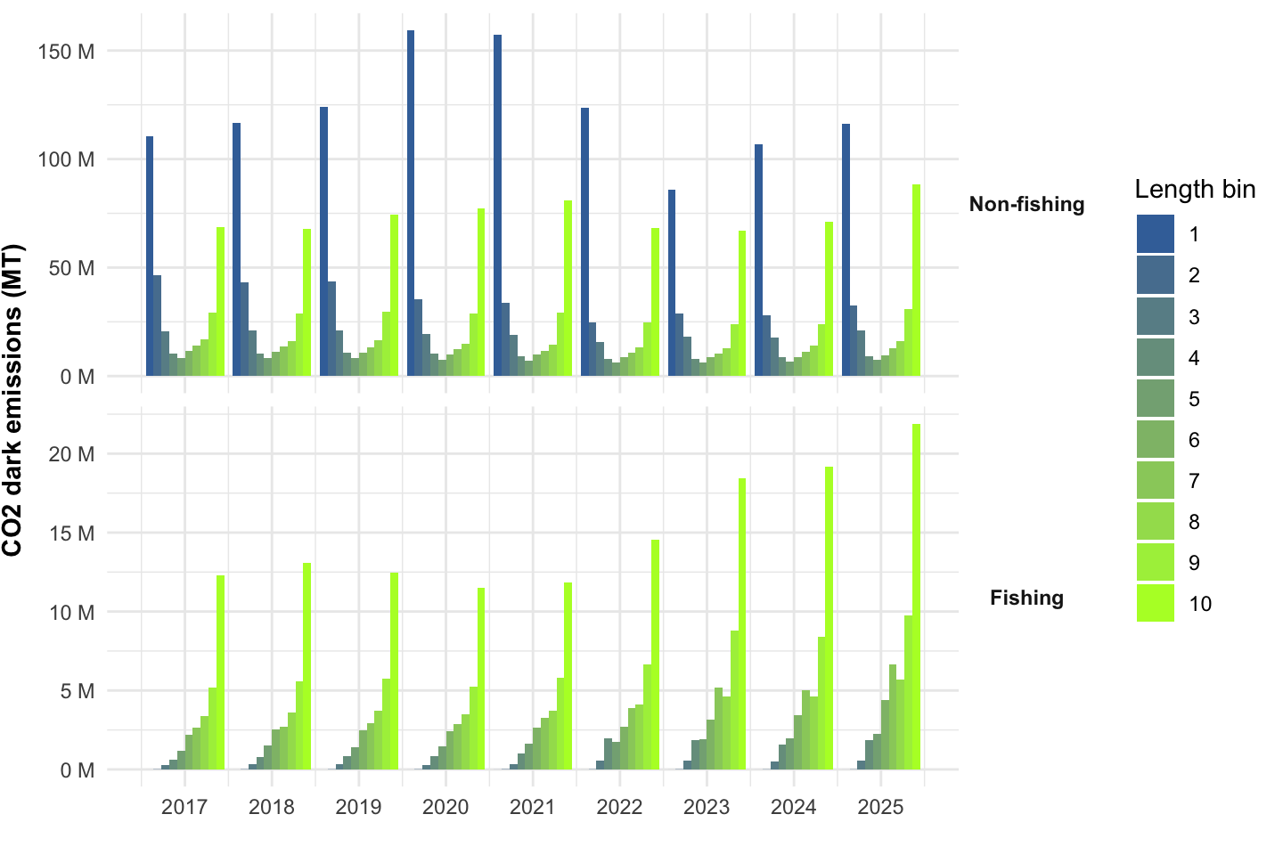
We can also explore how dark emissions are distributed by vessel type and across the time range. Figure 2.9 shows that emissions from fishing vessels, and the relationship between small and large fishing vessels, have been more consistent over the years, despite a significant decrease in the largest fraction at the beginning of the time series, followed by stabilization and a slight increase in recent years.
For non-fishing vessels—which account for the majority of emissions (Table 2.3)—there are clearer changes in both the relationship between small and large vessels and their emissions over time. Notably, there has been an inversion in the proportion of emissions between small and large non-fishing vessels, with a more significant reduction in emissions from larger vessels—possibly due to higher AIS adoption of that group—than from smaller ones. In recent years, smaller vessels have accounted for a larger proportion of emissions.
| year | fishing | emissions_co2_mt | emissions_co2_dark_mt |
|---|---|---|---|
| 2017 | FALSE | 795385087 | 336786470 |
| 2017 | TRUE | 28833568 | 27815439 |
| 2018 | FALSE | 829892604 | 337460801 |
| 2018 | TRUE | 31525370 | 30120248 |
| 2019 | FALSE | 850662483 | 353021318 |
| 2019 | TRUE | 33419302 | 29958277 |
| 2020 | FALSE | 844915658 | 375961201 |
| 2020 | TRUE | 34139044 | 28181265 |
| 2021 | FALSE | 904599809 | 372802527 |
| 2021 | TRUE | 36498797 | 30269459 |
| 2022 | FALSE | 957187349 | 304373993 |
| 2022 | TRUE | 47337049 | 36216068 |
| 2023 | FALSE | 995087906 | 269927534 |
| 2023 | TRUE | 59161261 | 44493203 |
| 2024 | FALSE | 1074913457 | 296863046 |
| 2024 | TRUE | 64284518 | 44716957 |
| 2025 | FALSE | 1122295153 | 344136064 |
| 2025 | TRUE | 67117600 | 53047846 |
2.2.3 Spatial maps of emissions
Next we can look at spatial maps of global emissions by the AIS-broadcasting fleet and by the dark fleet. For each 1x1 degree pixel (the spatial resolution of the dark fleet model), we aggregate emissions separately for each pollutant for 2025.
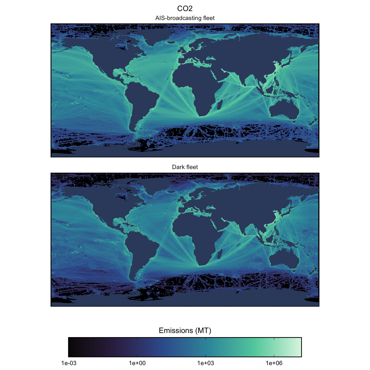
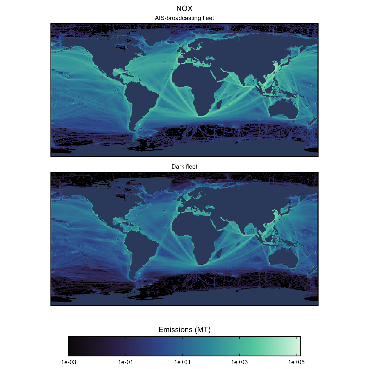
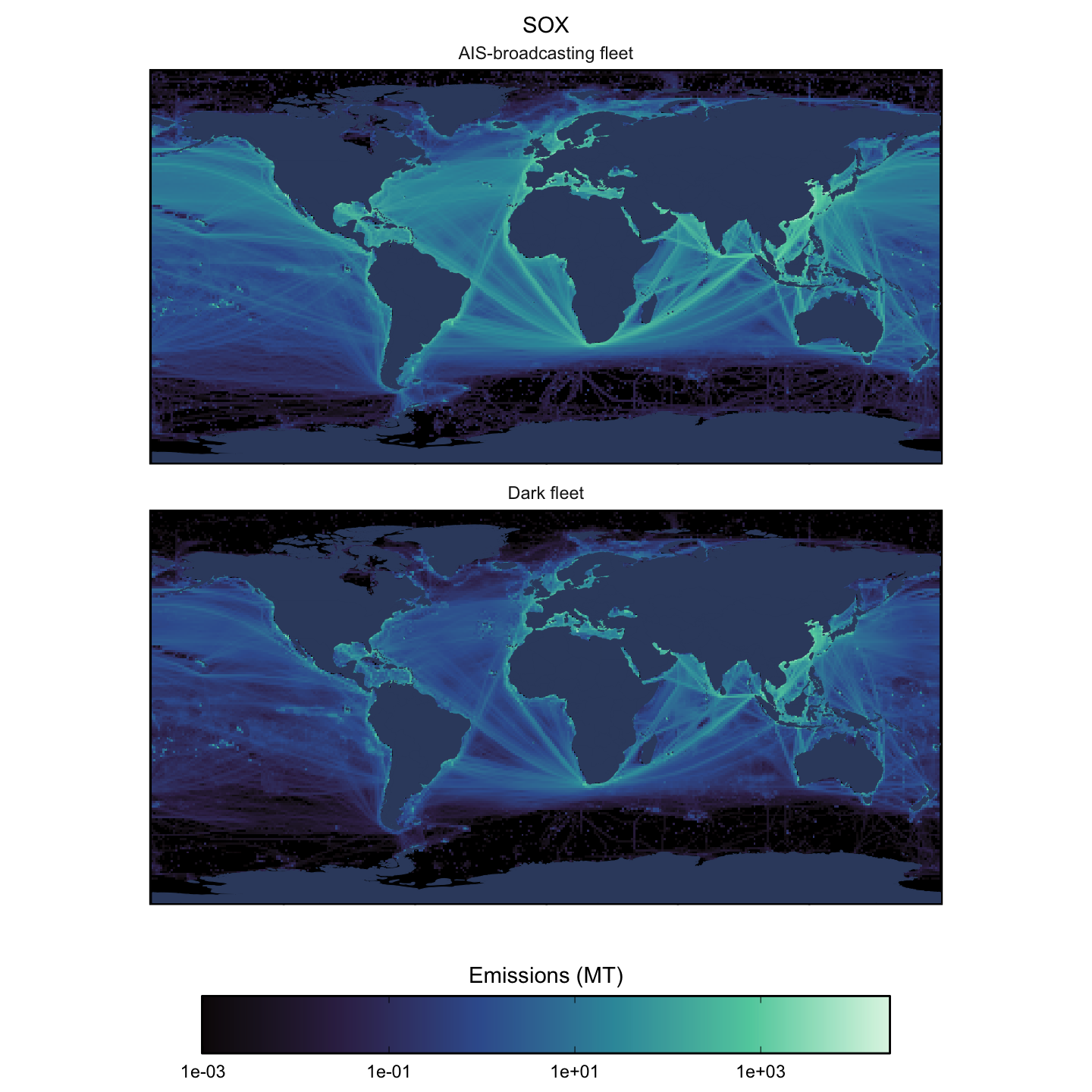
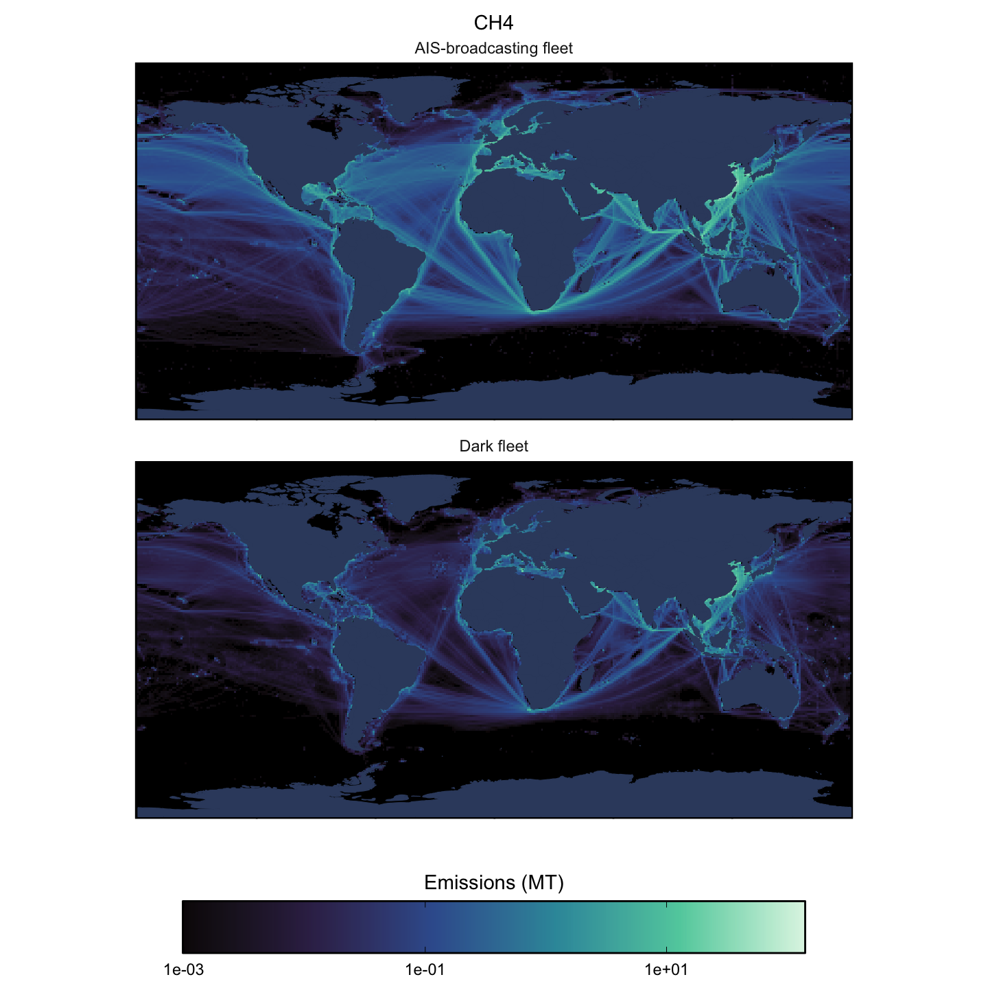
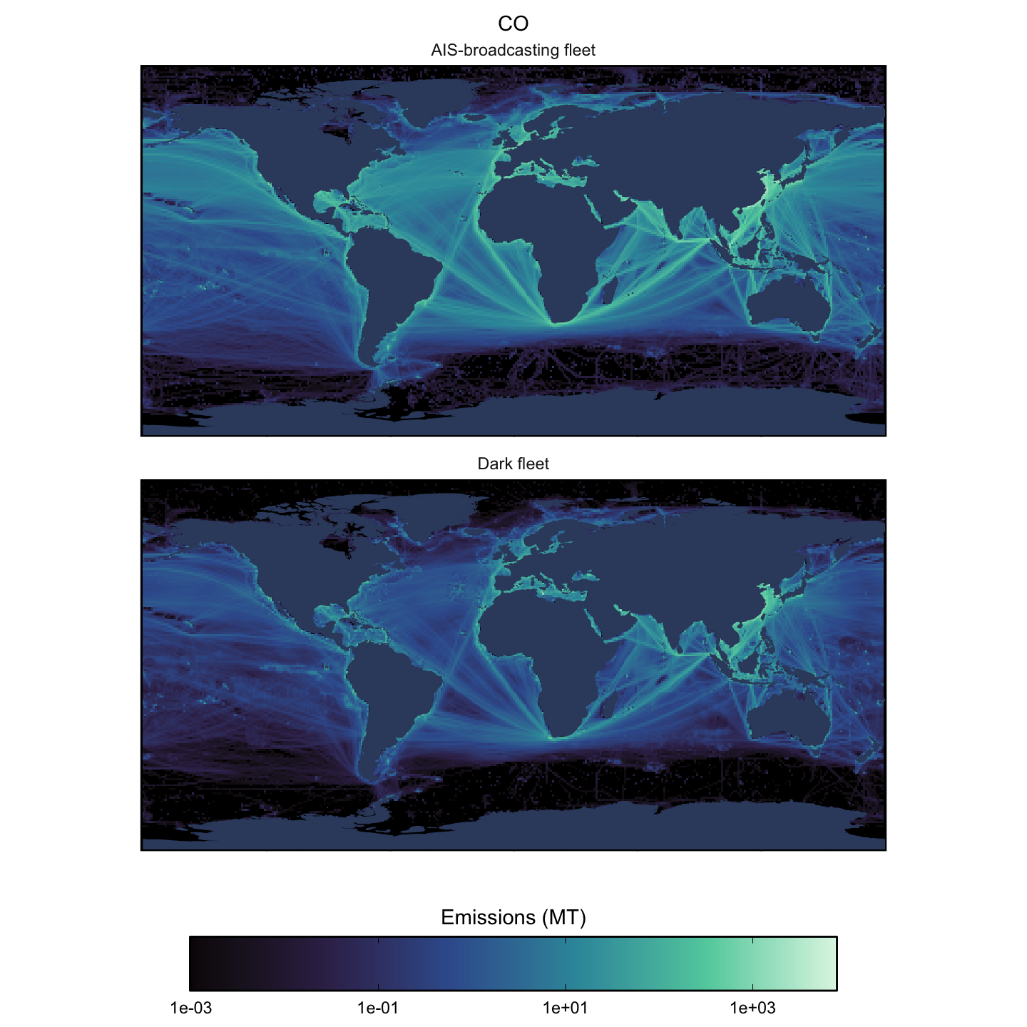
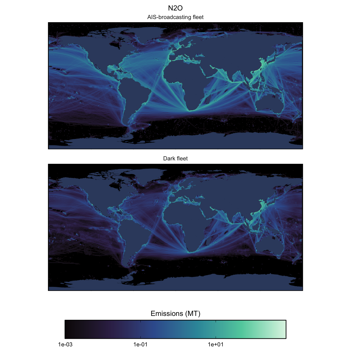
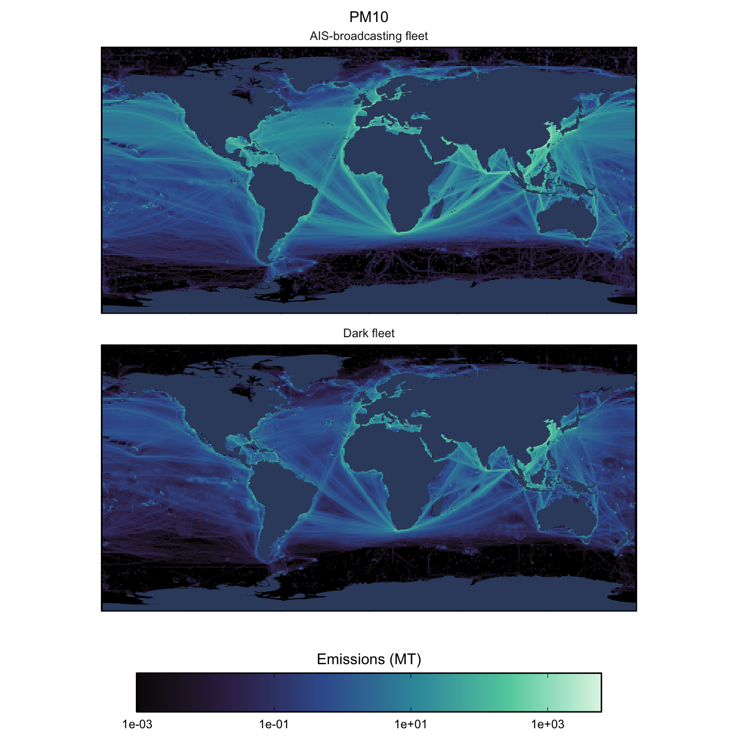
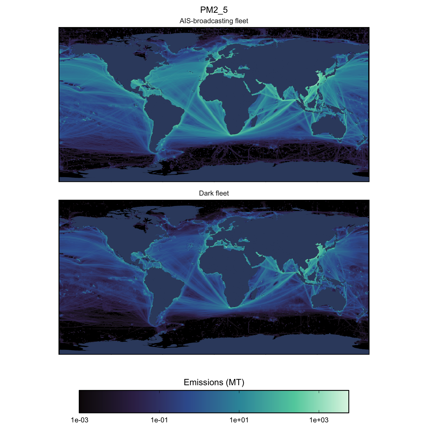
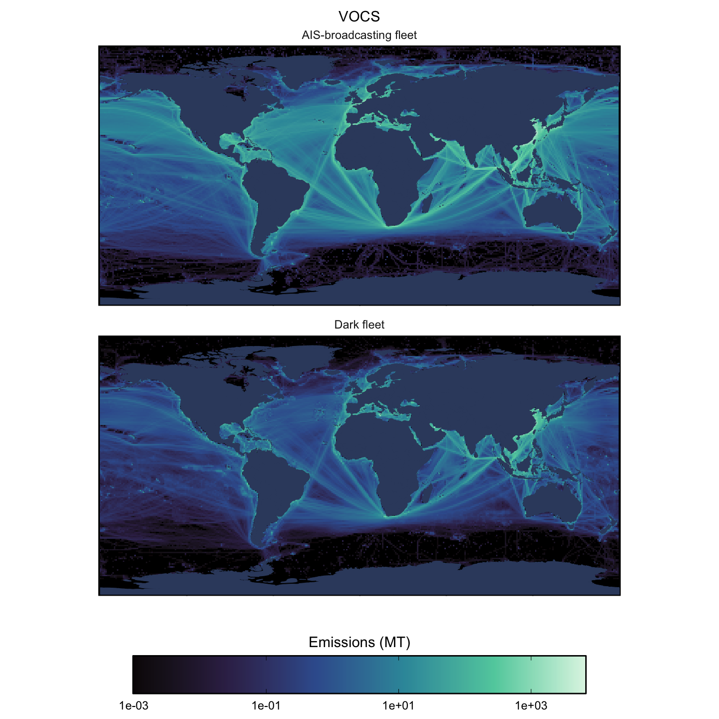
The spatial distribution of dark emissions heavily depends on how areas outside the S1 footprint are handled. While the updated KNN approach improves upon the use of global ratios by capturing greater temporal and spatial variability, there is still room for refinement in this area, as detailed in the section about potential model refinements. The assignment of ratios affects not only the spatial distribution of emissions in areas not covered by S1 but also the total emission estimates. When examining the origin of emissions—whether pixel ratios were directly assigned based on S1 detections or determined using KNN—it becomes evident that most dark emissions originate from areas not covered by S1. This is expected, as S1 primarily covers coastal areas, leaving the majority of the ocean unobserved. As shown in Table 2.4, approximately 65–73% of emissions are attributed to areas outside the footprint. On the contrary, when considering relative values by area, we see higher emission densities within the S1-covered zones, as most detections occur closer to the coast.
Given the significant contribution of dark emissions from pixels outside the footprint—and from those with null values within the footprint—it is important to highlight how these contribute to the uncertainty in the total estimates, as they rely entirely on extrapolated ratios. Therefore, among dark emissions, it is essential to differentiate between emissions inside and outside the S1 footprint and assess uncertainty independently. This distinction underscores the importance of improving methodologies for handling emissions outside the footprint, given their substantial influence on total estimates and the associated uncertainties, which must be minimized.
| year | s1_footprint | emissions_co2_dark_mt | emissions_by_pixel | percentage_of_total |
|---|---|---|---|---|
| 2017 | outside | 206069250 | 124.24289 | 56.51897 |
| 2017 | within | 158532658 | 566.17593 | 43.48103 |
| 2018 | outside | 207592444 | 122.92334 | 56.47528 |
| 2018 | within | 159988606 | 532.07336 | 43.52472 |
| 2019 | outside | 215664609 | 127.40759 | 56.31230 |
| 2019 | within | 167314986 | 532.06912 | 43.68770 |
| 2020 | outside | 245935843 | 146.57185 | 60.85375 |
| 2020 | within | 158206623 | 504.82668 | 39.14625 |
| 2021 | outside | 238317052 | 138.67470 | 59.12518 |
| 2021 | within | 164754935 | 508.76041 | 40.87482 |
| 2022 | outside | 198516980 | 108.08728 | 58.28619 |
| 2022 | within | 142073081 | 506.24853 | 41.71381 |
| 2023 | outside | 161413844 | 85.88881 | 51.33689 |
| 2023 | within | 153006894 | 547.55613 | 48.66311 |
| 2024 | outside | 187209407 | 98.58227 | 54.80690 |
| 2024 | within | 154370595 | 531.99137 | 45.19310 |
| 2025 | outside | 209263344 | 107.91682 | 52.68676 |
| 2025 | within | 187920566 | 650.85224 | 47.31324 |
2.2.4 Regional trends
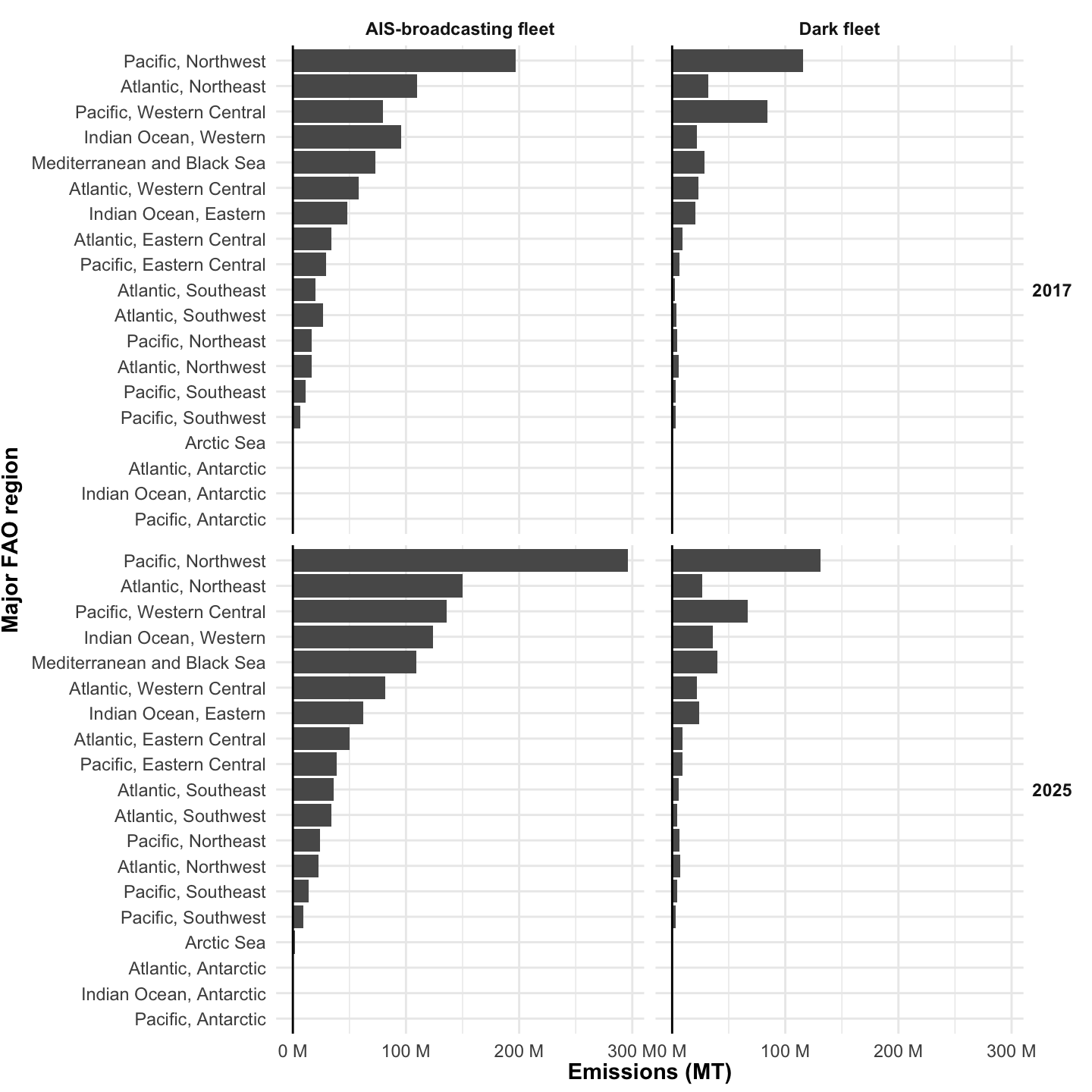
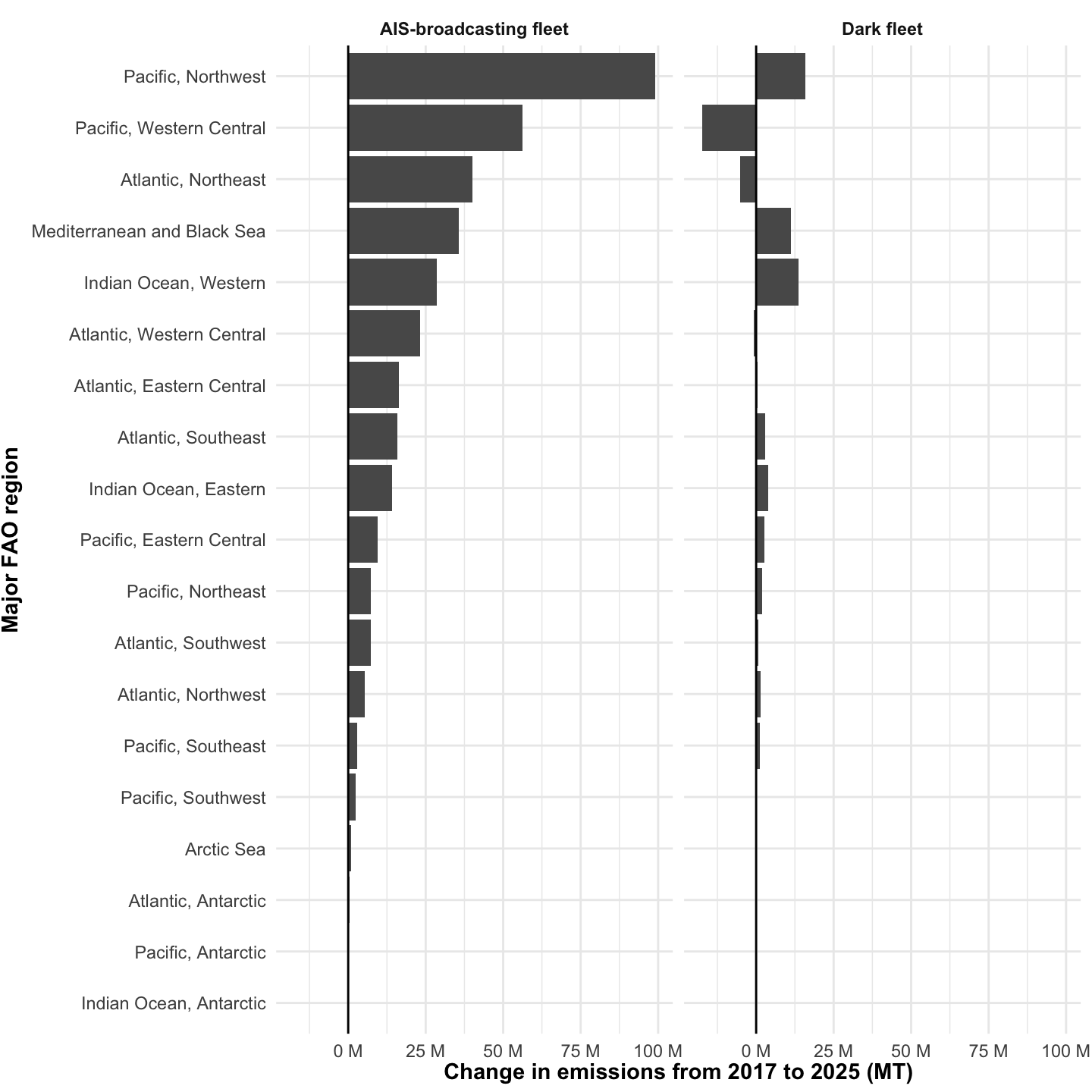
We can also look at broader regional trends in emissions estimates by looking at Major FAO Regions. There are 19 major FAO regions (Figure 2.19).
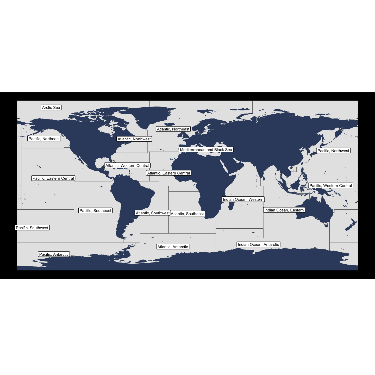
For each region, we summarize emissions for both the AIS-broadcasting and dark fleets. Below we do this focused on summarizing annual emissions of CO2, and focusing on 2017 and 2025 (the first and last years of our dark fleet time series data) (Figure 2.20, Figure 2.21).
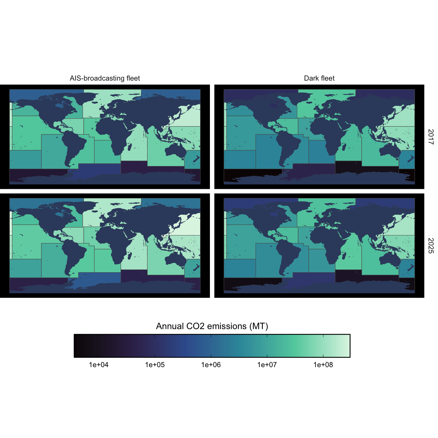
Finally we look at the change in CO2 emissions between 2017 and 2025 for each of these regions (Figure 2.22).
2.3 Available data tables (BigQuery)
This section documents the main result table produced by the dark fleet emissions model. As with the AIS tables (Section 1.4), it lives in the proj_ocean_ghg BigQuery dataset with a model-version suffix (currently _v20260714), e.g. proj_ocean_ghg.s1_time_gridded_dark_fleet_model_v20260714. Emissions columns are in metric tonnes (mt) and cover the same pollutants as the AIS model (CO₂, CH₄, N₂O, NOₓ, SOₓ, CO, VOCs, PM2.5, PM10). The delivered Climate TRACE dark fleet product built from this table is documented in Chapter 3.
2.3.1 s1_time_gridded_dark_fleet_model — gridded dark + AIS emissions
The core dark fleet model output. One row per time × 1° grid cell × fishing status × vessel size class. For each cell it carries the AIS-broadcasting-fleet emissions, the Sentinel-1 detection ratios used to scale them up, and the resulting modeled dark (non-broadcasting) emissions (the *_dark_mt columns). The time grain is set by the model’s temporal-extrapolation unit (currently monthly).
| Column | Description |
|---|---|
time |
Time bin (currently month; timestamp truncated to the extrapolation unit). |
lon_bin / lat_bin |
Lower-left corner of the 1° grid cell. |
fishing |
Whether the vessels are of a fishing class. |
length_size_class_percentile |
Vessel length size-class bin, defined from percentile cut-points of Sentinel-1-detected vessel lengths. |
number_dark_detections |
Count of Sentinel-1 detections not matched to AIS (dark) in the cell. |
number_ais_detections |
Count of Sentinel-1 detections matched to AIS in the cell. |
ratio_dark_to_ais_detections |
Dark-to-AIS detection ratio for the cell (within-footprint; filled from kNN neighbors where directly missing). |
global_time_ratio_dark_to_ais_detections |
Fallback ratio derived from kNN neighbors outside the S1 footprint, used where the cell has no within-footprint ratio. |
emissions_{co2,ch4,n2o,nox,sox,co,vocs,pm2_5,pm10}_mt |
AIS-broadcasting-fleet emissions of each pollutant in the cell (mt). |
emissions_{co2,ch4,n2o,nox,sox,co,vocs,pm2_5,pm10}_dark_mt |
Modeled dark-fleet emissions of each pollutant (AIS emissions × detection ratio) (mt). |
null_ratio |
TRUE where no detection ratio was available (cell outside the dark-estimation domain); its *_dark_mt values are an explicit 0 rather than an estimate. |
The delivered Climate TRACE dark fleet product built by summing this table over all cells (climate_trace_schema_dark_fleet, with its confidence and uncertainty companions) is documented in Chapter 3.