1 AIS-based emissions model
1.1 Methods
1.1.1 Model Overview
We estimate emissions using an engineering bottom-up approach based on AIS data, vessel characteristics, and emissions conversion factors from the literature. The model follows the methodology of the 2020 IMO “Fourth Greenhouse Gas Study” (Faber and Xing (2020)) and the 2017 ICCT “Greenhouse Gas Emissions From Global Shipping” study (Olmer et al. (2017)), applied to the GFW data.
From a high level, we calculate emissions as follows:
For each individual AIS message (ping), we calculate the main engine energy use, auxiliary engine energy use, and boiler energy use (each in kilowatt-hours), each of which is a function of vessel characteristics, speed, and the time since the previous ping.
For each engine (main, auxiliary, and boiler), we assign each vessel an emissions factor (EF, in g/kWh) for each of nine pollutants (CO2, CH4, N2O, NOX, SOX, CO, PM10, PM2.5, and VOCs). These EFs come from two distinct families, described precisely in the emissions factor sections below: SFC-derived EFs (CO2, SOX, PM10, and PM2.5), whose g/kWh values are constructed from an explicit model of each engine’s specific fuel consumption (SFC) and the properties of the fuel burned, using the equations and tables of Faber and Xing (2020); and lookup-table EFs (NOX, CO, CH4, N2O, and VOCs), which are taken directly from published g/kWh tables (the appendices of Olmer et al. (2017) for NOX, CO, CH4, and N2O, and Appendix M of Faber and Xing (2020) for VOCs). These family names describe each factor’s provenance — how its g/kWh value is built — not the fuel-based versus energy-based application classification used by Faber and Xing (2020); see Section 1.1.2.2 for how the two map onto each other.
For each pollutant and ping, we multiply each engine’s energy use by its EF (applying the appropriate load-dependent correction to the main engine term; see below) and sum across the main, auxiliary, and boiler engines to get ping-level emissions.
In parallel, we compute fuel consumption for every ping as a tenth quantity, using the same machinery with the blended SFC (g fuel/kWh) in place of an emissions factor (see Section 1.1.6). Fuel consumption is carried through all internal tables, but is not part of the delivered Climate TRACE schema.
With ping-level emissions, we aggregate emissions by vessel, by voyage, by port stay, by time, by space, etc.
1.1.2 Main engine
1.1.2.1 Main engine energy use
Based on Faber and Xing (2020) (page 64), main engine energy use (in killowatt-hours) is calculated as follows:
\[\text{Main Engine Energy Use}_{kWh} = \text{Hours} \times \text{Load Factor} \times \text{Main Engine Power}_{kW} \] Where hours comes from each individual AIS message, main engine power (kW) comes from the vessel characteristics dataset, and the load factor comes from the product of several correction factors (CFs):
\[\text{Load Factor} = \text{Speed-power CF} \times \text{Hull Fouling CF} \times \text{Weather CF} \times \text{Draft CF}\] Where: - hull fouling CF is 1.07, reflecting a 7% increase in resistance as described in Olmer et al. (2017) and Faber and Xing (2020) (see page 17 and Annexes page 270, respectively) - weather CF is a correction factor based on weather conditions, varying with the distance to shore. This factor is set at 1.1 for nearshore activity (≤5 nm from shore) to account for a 10% increase in resistance, and 1.15 for offshore activity (>5 nm), reflecting a 15% increase in resistance, as described in the Olmer et al. (2017) and Faber and Xing (2020) (see pages 18 and 270, respectively). - draft CF is extracted from the average draught by sector as reported in Olmer et al. (2017) (see Table 13 on page 20). Weights were applied by vessel type based on fuel consumption data from the Faber and Xing (2020) (see Annex 1, Figure 4), since fuel consumption values by type are proportionally related to emissions. This weighted average provided a final estimate of 0.85. speed-power CF is defined as \((\text{speed}_{knots} / {\text{design\_speed}_{knots}}) ^3\), with the additional stipulation that this ratio should not exceed 1:
\[\text{Speed-power CF} = \begin{cases} 1 & \text{if } \frac{\text{speed}_{knots}}{\text{design\_speed}_{knots}} > 1, \\ \frac{\text{speed}_{knots}}{\text{design\_speed}_{knots}} & \text{otherwise} \end{cases}\]
In this equation, speed is the AIS-broadcast instantaneous speed when one hour or less has elapsed since the previous message (we assume activity within the past hour traveled at a similar speed). For longer gaps we use the implied speed, which is more reliable over longer intervals and is calculated as the distance from the last position divided by the hours since the last position. Design speed comes from a bespoke machine learning model developed by GFW to infer design speed using a model trained on registry-derived values(see Section 1.1.9).
As a last step, we ensure that the final load factor (the product of the above correction factors) does not exceed a value of 0.98, as recommended by Faber and Xing (2020) (see page 272).
\[\text{Load Factor} = \begin{cases} 0.98 & \text{if (Load Factor)} > 0.98, \\ \text{Load Factor} & \text{otherwise} \end{cases}\]
1.1.2.1.1 Adjustments for fishing vessels
For fishing vessels, we adjust the main engine load factor based on the relationships published by Coello et al. (2015) (and later used by Sala et al. (2018)).
- For fishing vessels of class
trawlersanddredge_fishing, when they are actively fishing we assign a main engine load factor of 0.75. The intuition is that for these vessel types, even if they are moving slowly, their engines can be exerting tremdeous power while they are actually fishing with depolyed gear. - For all fishing vessels, we limit the main engine load factor so that it falls between 0.2 and 0.9
1.1.2.1.2 Low-load emissions adjustments
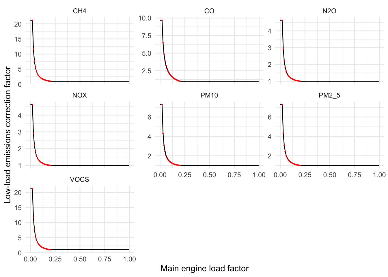
Additionally, for the main engine we apply low-load emissions correction factors based on the EPA’s 2020 Ports Emissions Inventory Guidance U.S. Environmental Protection Agency (2020) (which were the basis of Table 20, page 74, of @FourthIMOGHGStudy2020 ). Main engines operating during propulsion at very low loads below 20% operate inefficiently, and emit more of certain pollutants. Table 3.10 from the EPA report provides a lookup table of low-load emissions correction factors which vary based on the exact engine load and for each pollutant. Low-load correction factors are provided for a range from <=2% through >=20% in increments of 1%; if the engine load is <= 2%, it receives the correction factor corresponding to <=2%; if the load is greater than >=20%, it receives a correction factor of 1; if the load corresponds perfectly to a value in the table, it receives the corresponding correction correction factor; if the load falls between two values in the table, we linearly interpolate between those values.
Following Table 20 of Faber and Xing (2020) (see the table footnote on page 74), we do not apply these correction factors to CO2, SOX, or fuel consumption. These quantities vary directly with fuel consumption, so their low-load behavior is instead captured explicitly by the load-dependent specific fuel consumption (SFC) correction described in Section 1.1.2.2, exactly as in Faber and Xing (2020). All other pollutants (NOX, CO, CH4, N2O, VOCs, PM10, and PM2.5) receive the EPA low-load correction factors. Note one documented approximation: the PM10 and PM2.5 factors depend on fuel sulphur content and SFC in magnitude (see Section 1.1.2.2), but they are energy-based factors in the classification of Faber and Xing (2020), and — consistent with both that classification and EPA practice — their low-load behavior is handled by the EPA correction factors rather than the SFC correction.
In Figure 1.1 we can see what the low-load correction factors are for each pollutant in our analysis, each of which vary by main engine load (which falls between 0 and 1).
1.1.2.2 Main engine emissions factors
Main engine emissions for each pollutant are determined by multiplying each pollutant’s emissions factor (EF, g/kWh) by the main engine energy use. The emissions factors used throughout the model — for the main engine, the auxiliary engine, and the boiler alike — come from two distinct families with different provenance. The subsections below describe both families in full for the main engine; auxiliary engine and boiler EFs are built from the same two families, with their device-specific details (SFC values, lookup-table sources, and turbine handling) given in Section 1.1.3.6. The two families are:
- SFC-derived EFs — CO2, SOX, PM10, and PM2.5 (plus the fuel consumption output itself; see Section 1.1.6). These are constructed from an explicit model of the engine’s specific fuel consumption (SFC, g fuel/kWh) and the properties of the fuels burned, using the equations and tables of Faber and Xing (2020).
- Lookup-table EFs — NOX, CO, CH4, and N2O, taken directly from the g/kWh lookup tables in Appendix E (Table 55, page 38) of Olmer et al. (2017); and VOCs (NMVOC), taken from Appendix M (Table 61, page 414) of Faber and Xing (2020).
A note on terminology. Faber and Xing (2020) (page 72) classifies emissions factors by how they are applied: fuel-based EFs (\(EF_f\), g pollutant per g fuel, multiplied by fuel consumption) cover only CO2, SOX, and black carbon (which we do not model), while energy-based EFs (\(EF_e\), g pollutant per kWh, multiplied by engine energy use) cover every other pollutant — including PM10 and PM2.5, whose g/kWh factors (Equations 16–17, page 75) nonetheless depend on the fuel’s sulphur content and the engine’s SFC. Our model expresses every EF in g/kWh and multiplies it by engine energy use, and this is consistent with the IMO treatment for all pollutants: for CO2 and SOX we fold the fuel-based \(EF_f\) together with the SFC into an equivalent g/kWh form (algebraically identical, since fuel consumption is SFC × energy use), and for PM10 and PM2.5 we use the IMO energy-based equations directly. The two families above therefore describe each factor’s provenance — whether its g/kWh value is built from SFC and fuel properties, or read from a published lookup table — and deliberately avoid reusing the IMO’s application terms, since PM10 and PM2.5 are SFC-derived in provenance but energy-based in the IMO’s classification.
1.1.2.2.1 Engine classification
Both families are keyed to the same per-vessel engine classification. Based on engine type (oil/reciprocating, gas, or turbine) and engine RPM, each vessel’s main engine is assigned to one of four buckets: slow-speed diesel (SSD, <300 RPM), medium-speed diesel (MSD, 300–900 RPM), high-speed diesel (HSD, >900 RPM), or turbine. Note that vessels whose registry engine type is Gas denote gas-turbine propulsion ships, not LNG-fueled ships (see §2.1.5 of Olmer et al. (2017); we verified empirically that ~99% of these vessels burn distillate fuel), so they take the turbine factors throughout. No vessel is assigned LNG-fuel emissions factors, because the only per-vessel fuel-type field available to us is an untrusted model prediction (see Section 1.1.10 for the implications). Each engine is also assigned a build-year generation following Table 19 of Faber and Xing (2020): generation 1 (built ≤1983), generation 2 (1984–2000), or generation 3 (≥2001).
1.1.2.2.2 SFC-derived emissions factors: CO2, SOX, PM10, PM2.5
The foundation of the SFC-derived EFs is the baseline specific fuel consumption (\(SFC_{base}\), in g fuel per kWh) from Table 19 (pages 70–71) of Faber and Xing (2020), which tabulates SFC by engine bucket, build-year generation, and fuel (HFO and MDO). For main engines, these range from 165–225 g/kWh for diesel engines (newer and slower engines are more efficient) and are 305 (HFO) / 300 (MDO) g/kWh for turbines (the gas-turbine row of Table 19; no generation dependence). Auxiliary engines use the Table 19 auxiliary-engine SFC by build-year generation, and boilers use a fixed SFC of 340 (HFO) / 320 (MDO) g/kWh (the steam-boiler row of Table 19; constant, with no generation dependence).
Because we do not have reliable per-vessel fuel-type information, we use a fixed fuel-mix convention for oil/reciprocating engines: one-third HFO, one-third MDO, and one-third MDO in Emissions Control Areas (ECA), i.e. a \((\text{HFO} + 2 \times \text{MDO})/3\) blend. This mirrors the convention used throughout our lookup-table factors, which average across the HFO, distillate, and 2015+ ECA columns of the Olmer et al. (2017) appendix tables. The associated fuel sulphur contents are 2.7% (HFO, the pre-2020 global average), 0.14% (MDO), and 0.1% (ECA MGO, the MARPOL Annex VI ECA limit in force since 2015), consistent with the fuel sulphur assumptions of Olmer et al. (2017) and Table 22 (page 75) of Faber and Xing (2020). Turbine and gas-turbine vessels burn distillate rather than the HFO blend, so their sulphur-driven EFs (SOX, PM10, PM2.5) are computed over the two MDO terms only, with the HFO term dropped. The rationale for using a fixed blend rather than per-vessel fuel assignment, and a quantified sensitivity analysis of how much this assumption can matter for each pollutant, are given in Section 1.1.8.
The individual SFC-derived EFs are then:
- CO2: the SFC multiplied by the fuel-based carbon EF (\(EF_f\), g CO2 per g fuel) of each blend component, from Table 21 (page 74) of Faber and Xing (2020) (which takes them from the IMO’s 2018 EEDI Guidelines): 3.114 for HFO and 3.206 for MDO.
\[EF_{CO_2} = \frac{SFC_{HFO} \times 3.114 + 2 \times SFC_{MDO} \times 3.206}{3}\]
- SOX: Equation 15 (page 74) of Faber and Xing (2020), applied to each blend component and averaged. The factor 2 is the molecular weight ratio of SO2 to sulphur, and 0.97753 is the fraction of fuel sulphur converted to SOX (the remainder becomes sulphate aerosol, counted as particulate matter); \(S\) is the fuel sulphur content fraction:
\[EF_{SO_X} = SFC \times 2 \times 0.97753 \times S\]
- PM10: Equations 16 (HFO) and 17 (MDO/MGO) on page 75 of Faber and Xing (2020), applied to each blend component and averaged. These are the IMO’s energy-based PM equations — they yield \(EF_e\) in g/kWh directly, with the sulphur and SFC dependence embedded in the factor itself. The constant 7 is the molecular weight ratio between sulfate PM and sulphur, and 0.02247 is the proportion of fuel sulphur converted to sulfate PM (see page 76 of Faber and Xing (2020), citing the US EPA):
\[EF_{PM_{10}, HFO} = 1.35 + SFC \times 7 \times 0.02247 \times (S - 0.0246)\] \[EF_{PM_{10}, MDO/MGO} = 0.23 + SFC \times 7 \times 0.02247 \times (S - 0.0024)\]
- PM2.5: 92% of PM10, following page 76 of Faber and Xing (2020) (which cites EPA, 2019).
Because SOX, PM10, and PM2.5 depend on fuel sulphur content, each is computed under two sulphur regimes reflecting the IMO 2020 global sulphur cap (see 1) and the applicable regime is selected per ping based on its calendar year.
1.1.2.2.3 Load-dependent specific fuel consumption
Diesel engines are most efficient near their design load (roughly 75–80% of maximum continuous rating) and consume more fuel per kWh at low loads. Following Equation 11 (page 71) of Faber and Xing (2020) (adopted from the Third IMO GHG Study), the main engine SFC for internal-combustion (i.e., non-turbine) engines varies parabolically with the instantaneous engine load factor \(L\):
\[SFC = SFC_{base} \times (0.455 L^2 - 0.71 L + 1.28)\]
This correction is applied at the ping level to the fuel-proportional quantities (CO2, SOX, and fuel consumption) for internal-combustion main engines only; turbines use a constant SFC, and auxiliary engines and boilers also use constant SFC (see the Table 19 section, page 71, of Faber and Xing (2020)).1 This is precisely why the EPA low-load correction factors are not applied to CO2 or SOX (see the low-load section above): the low-load fuel penalty for these pollutants is captured here instead.
1.1.2.2.4 Lookup-table emissions factors: NOX, CO, CH4, N2O, VOCs
NOX, CO, CH4, and N2O emissions factors are taken directly from Appendix E (Table 55, page 38) of Olmer et al. (2017), averaging across the HFO, distillate, and 2015+ ECA fuel columns per the blend convention above. Year of build sets the IMO NOx tier (pre-2000, Tier I 2000–2010, or Tier II 2011+), and engine RPM sets the speed class within each tier. In Tiers I and II, engines rated between 130 and 2000 RPM use the RPM-dependent MARPOL Annex VI curve (\(0.94 \times 45 \times \text{RPM}^{-0.2}\) for Tier I, \(0.94 \times 44 \times \text{RPM}^{-0.23}\) for Tier II); engines below 130 RPM or at/above 2000 RPM, and all pre-2000 engines, receive fixed tabulated factors. Note that these NOx RPM breakpoints (130 and 2000 RPM) are specific to the MARPOL NOx curve and are distinct from the SSD/MSD/HSD engine buckets (300/900 RPM) used for the other factors. For turbine (and gas-turbine) engines, factors are averaged across the steam turbine and gas turbine rows. Where a vessel’s characteristics do not resolve to a single cell in the table, an average across the applicable cells is used.
VOCs (NMVOC) emissions factors are taken from Appendix M, Table 61 (page 414) of Faber and Xing (2020), which provides energy-based NMVOC factors by engine type: 0.632 g/kWh for slow-speed main engines, 0.527 g/kWh for medium- and high-speed main engines, and 0.105 g/kWh for gas and steam turbines. Auxiliary engines and boilers take their own Table 61 NMVOC factors: 0.421 g/kWh for auxiliary engines and 0.105 g/kWh for boilers (the boiler/steam-turbine row). Table 61’s values are identical across HFO, MDO, and LSHFO, so no fuel-blend weighting is needed and the factors carry no sulphur dependence.
Since none of the lookup-table factors depend on fuel sulphur content, they are identical in the pre- and post-2020 sulphur regimes.
1.1.3 Auxilliary engine and boiler
The model described in Faber and Xing (2020) assumes that while in service, a ship is operating in one of four defined phases: at berth, at anchor, maneuvering, or at sea.
For small vessels, we follow the recommendations from the 4th IMO study (page 68, Faber and Xing (2020)), where auxiliary engine power and boiler power are relative to main engine power. For larger vessels, aux_engine_power_kw and boiler_power_kw are defined based on vessel class and operational phase.
\[\text{Aux engine Energy Use}_{kWh} = \text{hours} \times \begin{cases} 0 & \text{if } \text{main\_engine\_power\_kw} \leq 150 \\ 0.05 \times \text{main\_engine\_power\_kw} & \text{if } \text{main\_engine\_power\_kw} \leq 500 \\ \text{aux\_engine\_power\_kw} & \text{otherwise} \end{cases}\]
\[\text{Boiler Energy Use}_{kWh} = \text{hours} \times \begin{cases} 0 & \text{if } \text{main\_engine\_power\_kw} \leq 150 \\ \text{boiler\_power\_kw} & \text{otherwise} \end{cases}\]
The inclusion of the four phases for larger vessels requires the use of Table 17 from the Faber and Xing (2020), including energy demand for the auxiliary engine and the boiler. However, this table expresses power demand based on vessel tonnage in different units. Since GFW has vessel size in GT, we needed to convert some of the values represented in DWT, TEU, and CBM to GT. Here, we present the approach followed to establish a direct size units relationship by vessel category.
1.1.3.1 DWT conversion
To establish the GT-DWT relationship, we used data containing both GT and DWT for each vessel. By assessing the relationship between these units, which mostly present linear relationships by vessel type, we defined a simple regression allowing us to derive conversion expressions with sufficient confidence from one unit to the other.
Such data was obtained through web scraping from open online sources, containing information for 464799 vessels on variables such as type, gt, dwt, length_m, beam_m, through which we could draw the size units relationship by vessel class.
Out of all vessel types, we only need to evaluate the tonnage relationship for several types in Table 17 from Faber and Xing (2020):
$ship_type
[1] "Bulk carrier"         "Chemical tanker"      "General cargo"
[4] "Oil tanker"           "Other liquids tanker" "Refrigerated bulk"
[7] "Ro-Ro"
In order to properly establish the size relationship, we need to group the categories from our dataset so they match the categories from Table 17. By doing so, we can evaluate each category’s relationship.
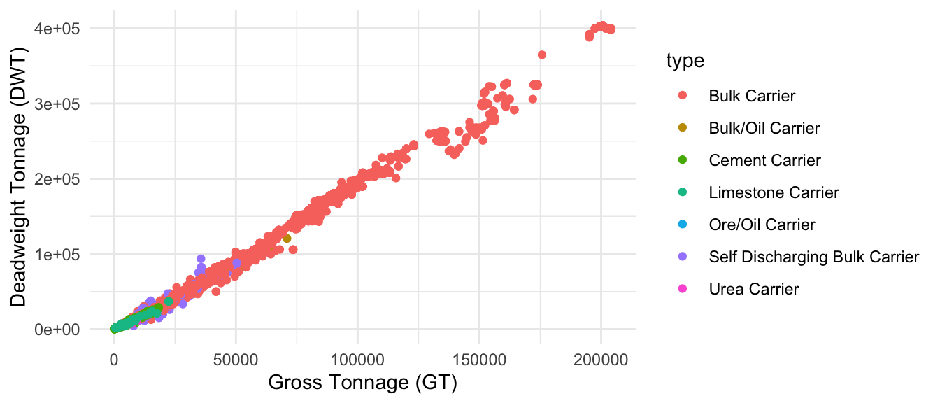
For instance, for Bulk carriers we have 7 categories which, according to Figure 1.2, present a linear relationship.
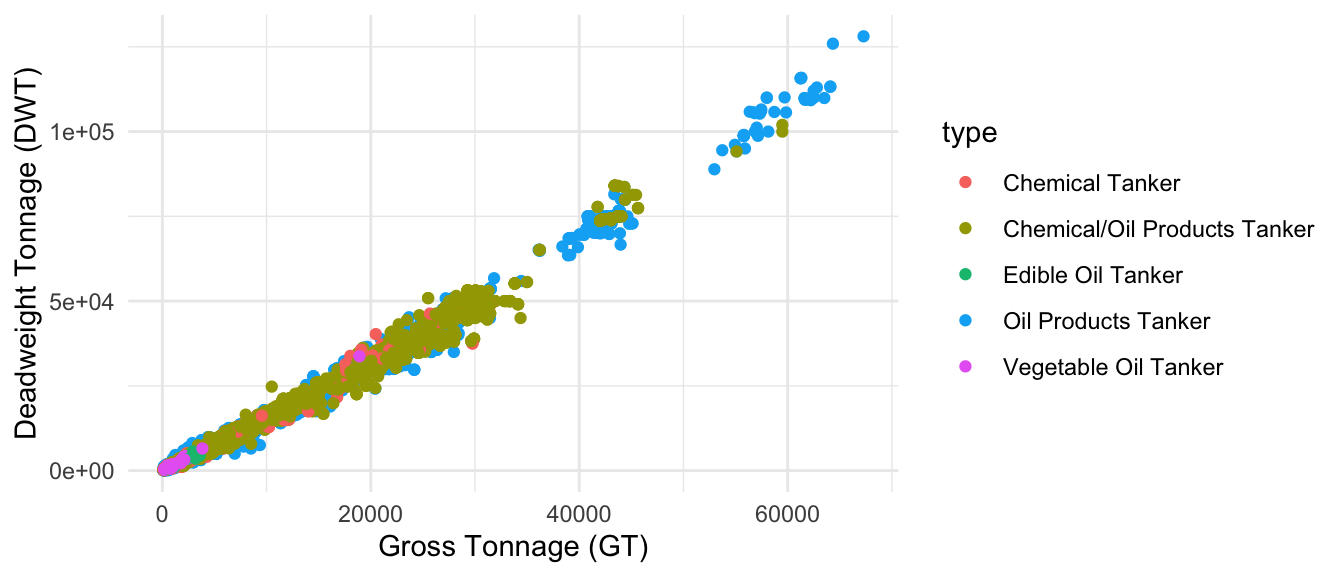
The same occurs for chemical tankers with 5 categories, as shown in Figure 1.3.
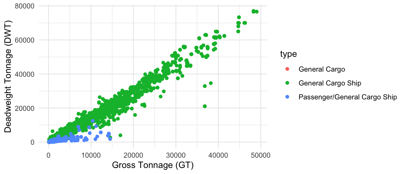
For general cargo, we have 3 categories. One of them, Passenger/General Cargo Ship, as seen in Figure 1.4, deviates from the linearity and may fall within the Ferry-pax only category from Table 17, so we will discart it.
Related to oil tankers, several vessel categories contain the label oil. However, most of them actually belong to chemical or bulk carriers. In this grouping, we will exclusively include crude oil tankers and bitumen Tankers.
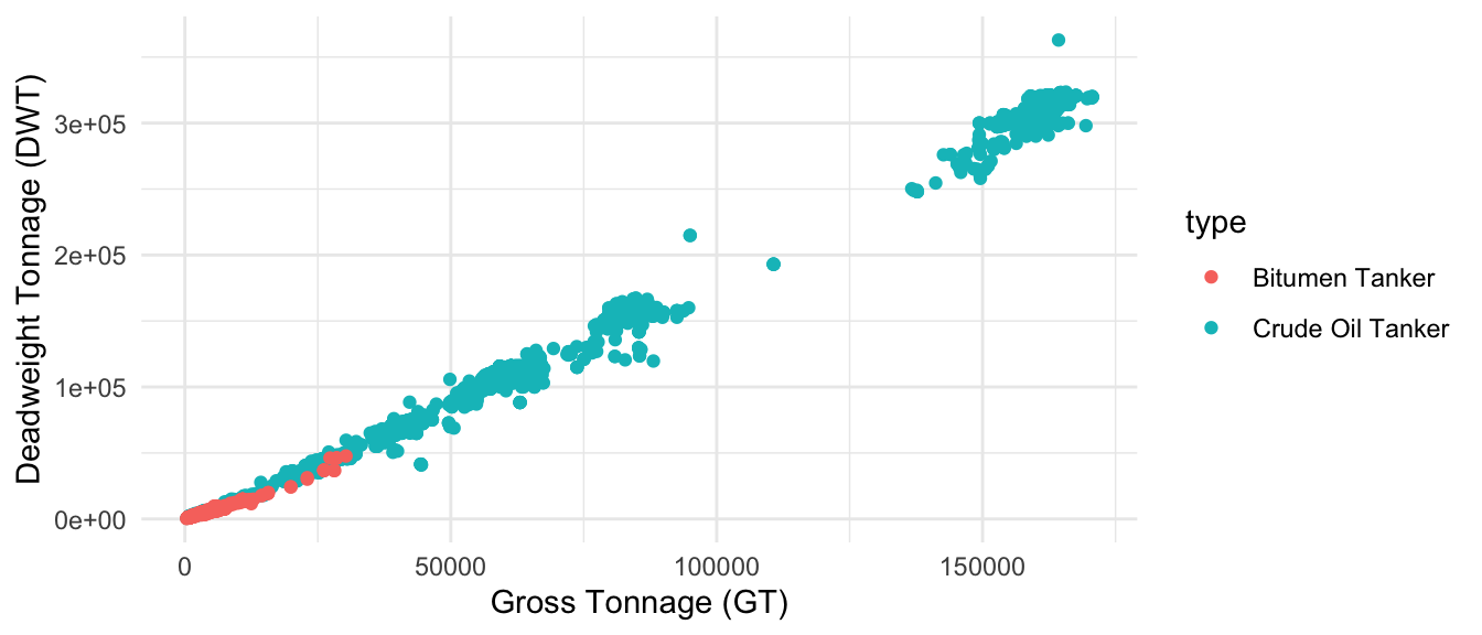
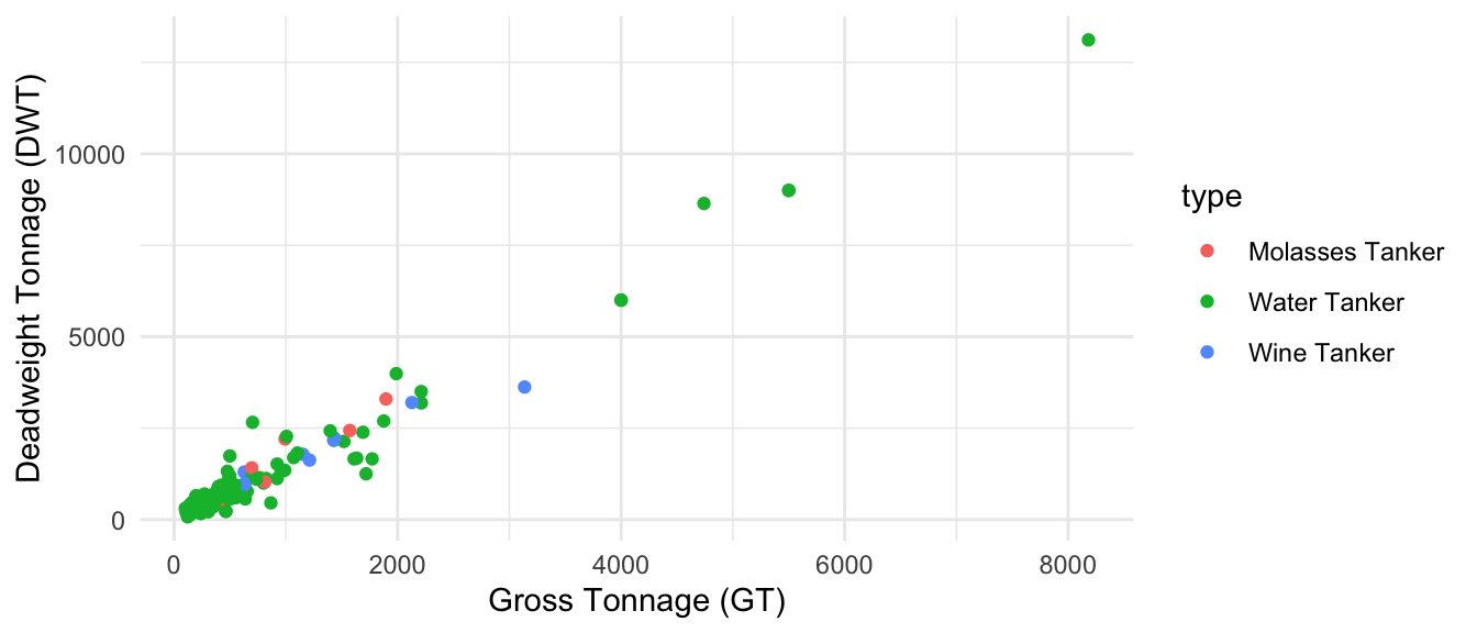
For the remaining liquid carriers, we will assign “Water Tanker”, “Wine Tanker” and “Molasses Tanker” from our table to the same category (Figure 1.6).
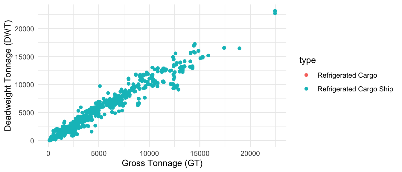
For refrigerated bulk, we have 2 categories, as shown in Figure 1.7.
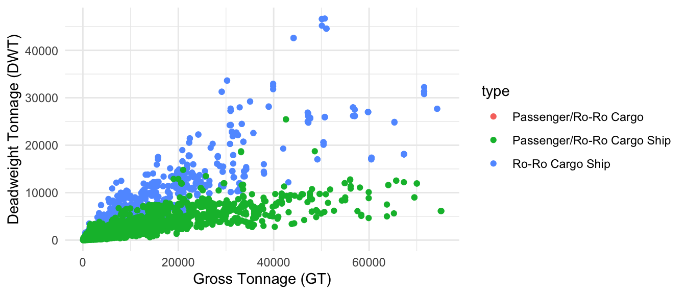
Lastly, for Ro ships, we have 3 categories, following distinct relationships as shown in Figure 1.8. Only Ro-Ro Cargo ships are the ones we are interested in, as the other two fall within the Ferry-RoPax category from Table 17.
With the defined equivalences between groups from Faber and Xing (2020) and groups from our dataset described above, we update the original dataframe to adjust the regressions. By fitting gross tonnage (GT) based on deadweight tonnage (DWT) and grouped type, we obtain the expressions explaining the relationship between both size units per vessel type, along with the performance metrics summarized in Table Table 1.1. We save this expression in a lm model fit object and used it later to update table 17.
| r.squared | adj.r.squared | sigma | statistic | p.value | df | logLik | AIC | BIC | deviance | df.residual | nobs |
|---|---|---|---|---|---|---|---|---|---|---|---|
| 0.9935724 | 0.9935717 | 2496.954 | 1325496 | 0 | 7 | -554797.7 | 1109613 | 1109694 | 374236342508 | 60024 | 60032 |
1.1.3.2 TEU conversion
TEU stands for Twenty-foot Equivalent Unit, which is a standard unit of measure used in the shipping industry to describe the capacity of container ships and terminals. One TEU represents the dimensions of a standard 20-foot long container. Therefore, TEU is used to quantify cargo capacity in terms of the number of 20-foot containers a vessel can carry. For example, a ship with a capacity of 10,000 TEU can carry 10,000 standard 20-foot containers.
For TEU, we obtain GT equivalents based on the design formulas for the calculation of key design vessel characteristics from Abramowski et al. (2018) as detailed below:
\[GT = -1097.4+11.049·TEU\]
1.1.3.3 CBM conversion
The size units of liquefied tankers represented as “CBM” refer to cubic meters (m³). This measurement indicates the volume capacity of the tankers, specifically how much liquefied gas (such as liquefied natural gas, LNG, or liquefied petroleum gas, LPG) they can carry.
For this unit conversion, we have not been able to find any large dataset to establish linear relationships, nor any publication defining expressions for unit conversion. The only available resource is the information from 23 vessels containing GT and CBM values, which allows to define a basic regression. This establishes the GT equivalence with intermediate to low confidence to update table 17 for gas tankers.
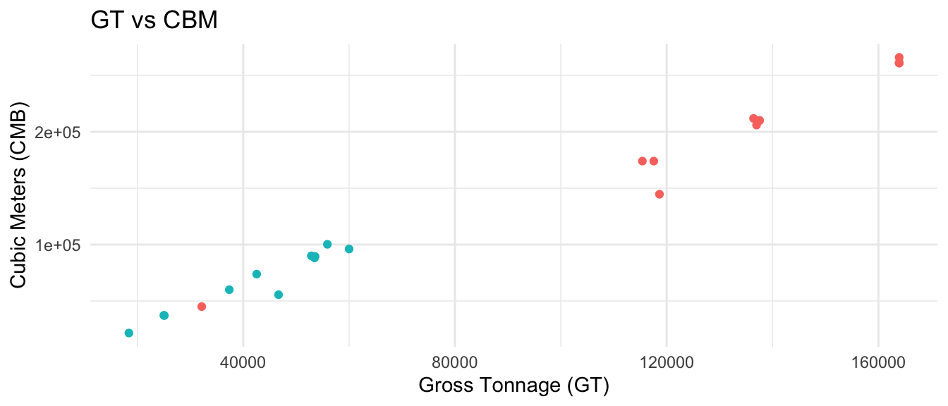
Here we see the model performance of GT as a function of CBM (Table 1.2).
| r.squared | adj.r.squared | sigma | statistic | p.value | df | logLik | AIC | BIC | deviance | df.residual | nobs |
|---|---|---|---|---|---|---|---|---|---|---|---|
| 0.982426 | 0.9815891 | 7253.543 | 1173.945 | 0 | 1 | -236.0421 | 478.0841 | 481.4906 | 1104891522 | 21 | 23 |
1.1.3.4 Updating table 17
Once we defined the relationship between GT and the other size units for each vessel class, we updated Table 17 from (Table 1.3). This allows us to incorporate the auxiliary engine and boiler power outputs per vessel type and operational mode into our AIS-based model.
| ship_type | size_lower | size_upper | size_units | size_lower_gt | size_upper_gt |
|---|---|---|---|---|---|
| Bulk carrier | 0 | 9999 | dwt | 0.000 | 7738.351 |
| Bulk carrier | 10000 | 34999 | dwt | 7738.864 | 20567.005 |
| Bulk carrier | 35000 | 59999 | dwt | 20567.518 | 33395.658 |
| Bulk carrier | 60000 | 99999 | dwt | 33396.171 | 53921.504 |
| Bulk carrier | 100000 | 199999 | dwt | 53922.017 | 105236.119 |
| Bulk carrier | 200000 | NA | dwt | 105236.632 | NA |
1.1.3.5 Mapping GFW vessel types to IHS vessel types
GFW’s vessel classification algorithm classifies each vessel as a particular ship type. Many GFW vessel types were designed to match perfectly to IHS ship types (e.g., oil tankers, container cargos); in these cases, we can use the adjusted Table 17 directly as a lookup table. In some cases, a single GFW vessel type may patch to multiple IHS ship types (e.g., the GFW vessel type passenger could correspond to Ferry-RoPax, Ferry-Pax only, or Cruise). In these cases, we take an evenly-weighted average across the mutliple vessel types it could match to. Table 1.4 shows this mapping and the weights assigned. With this, we update proj_ocean_ghg.vessel_info_v* by including the corresponding boiler and auxiliary engine power demand considering vessel size and class for each of the four operational phases. These operational phases depend on the speed, distance to shore, and distance to port of each individual AIS, all of which is known from our core underlying GFW data. This can then be fed into the model to provide more accurate emission estimates.
| gfw_vessel_class | tb17_ship_type | weights |
|---|---|---|
| bunker | Oil tanker | 1.00 |
| cargo.bulk_carrier | Bulk carrier | 1.00 |
| cargo.container | Container | 1.00 |
| cargo.general | General cargo | 1.00 |
| cargo.refrigerated | Refrigerated bulk | 1.00 |
| cargo.ro_ro | Ro-Ro | 1.00 |
| container_reefer | Refrigerated bulk | 1.00 |
| dive_vessel | Service - other | 0.50 |
| dive_vessel | Offshore | 0.50 |
| dredge_fishing | Miscellaneous - fishing | 1.00 |
| dredge_non_fishing | Service - other | 0.50 |
| drifting_longlines | Miscellaneous - fishing | 1.00 |
| driftnets | Miscellaneous - fishing | 1.00 |
| fish_factory | Miscellaneous - fishing | 1.00 |
| other_fishing | Miscellaneous - fishing | 1.00 |
| other_not_fishing | Miscellaneous - other | 0.50 |
| other_not_fishing | Service - other | 0.50 |
| other_purse_seines | Miscellaneous - fishing | 1.00 |
| other_seines | Miscellaneous - fishing | 1.00 |
| passenger | Ferry-RoPax | 0.33 |
| passenger | Ferry-pax only | 0.33 |
| passenger | Cruise | 0.33 |
| patrol_vessel | Service - other | 1.00 |
| pole_and_line | Miscellaneous - fishing | 1.00 |
| pots_and_traps | Miscellaneous - fishing | 1.00 |
| research | Service - other | 0.50 |
| research | Offshore | 0.50 |
| seismic_vessel | Service - other | 0.50 |
| seismic_vessel | Offshore | 0.50 |
| set_gillnets | Miscellaneous - fishing | 1.00 |
| set_longlines | Miscellaneous - fishing | 1.00 |
| specialized_reefer | Refrigerated bulk | 1.00 |
| squid_jigger | Miscellaneous - fishing | 1.00 |
| supply_vessel | Service - other | 0.50 |
| supply_vessel | Offshore | 0.50 |
| tanker.chemical | Chemical tanker | 1.00 |
| tanker.liquefied_gas | Liquefied gas tanker | 1.00 |
| tanker.oil | Oil tanker | 1.00 |
| tanker.other | Other liquids tanker | 1.00 |
| trawlers | Miscellaneous - fishing | 1.00 |
| trollers | Miscellaneous - fishing | 1.00 |
| tug | Service - tug | 1.00 |
| tuna_purse_seines | Miscellaneous - fishing | 1.00 |
| well_boat | Service - other | 1.00 |
1.1.3.6 Auxilliary engine and boiler emissions factors
Auxiliary engine and boiler emissions are determined by multiplying each pollutant’s emissions factor by the auxiliary engine or boiler energy use. The same SFC-derived versus lookup-table split described for the main engine (Section 1.1.2.2) applies here, with the same \((\text{HFO} + 2 \times \text{MDO})/3\) blend convention, the same sulphur contents, and the same two sulphur regimes:
- SFC-derived EFs (CO2, SOX, PM10, PM2.5, fuel consumption) are built from the auxiliary-engine and boiler \(SFC_{base}\) values in Table 19 (pages 70–71) of Faber and Xing (2020). Auxiliary engine SFC varies by build-year generation only (HFO: 225/205/195 g/kWh for generations 1/2/3; MDO: 210/190/185), with no RPM dependence. Boiler SFC uses the steam-plant (steam turbine and boiler) row of Table 19: a constant 340 g/kWh (HFO) / 320 g/kWh (MDO), with no generation dependence. Unlike the main engine, auxiliary engine and boiler SFC is constant with respect to load — the load-dependent SFC correction (Equation 11) applies to internal-combustion main engines only, per the Table 19 section (page 71) of Faber and Xing (2020). From these SFC values, CO2 (Table 21 carbon factors), SOX (Equation 15), PM10 (Equations 16–17), and PM2.5 (0.92 × PM10) are computed exactly as described for the main engine.
- Lookup-table EFs for NOX, CO, CH4, and N2O are taken from Appendix G (Table 57, page 52) of Olmer et al. (2017) for auxiliary engines and Appendix H (Table 58, page 53) for boilers, averaged across the HFO, distillate, and 2015+ ECA fuel columns. Auxiliary NOx factors additionally depend on the vessel’s engine tier, determined by year of build and engine RPM: pre-2000 vessels receive a single factor, while Tier I (2000–2010) and Tier II (2011+) vessels use RPM-dependent factors, with the MARPOL Annex VI curve applied for engines rated between 130 and 2000 RPM (the same breakpoints as the main engine). Boiler factors do not vary by NOx tier or RPM. The resolved numeric NOx factors (main engine, auxiliary, and boiler) are listed in Table 1.5, and the CO, CH4, and N2O factors in Table 1.6. VOCs factors come from Appendix M, Table 61 (page 414) of Faber and Xing (2020): 0.421 g/kWh for auxiliary engines and 0.105 g/kWh for boilers (the boiler/steam-turbine row).
Steam- and gas-turbine ships (registry engine types Turbine and Gas) have no separate auxiliary engines or boilers — their turbines supply auxiliary power and heat (see §2.4.1.1 of Olmer et al. (2017)) — so all of their auxiliary engine and boiler emissions factors are zero, for every pollutant.
\[\text{Aux engine emissions}_{g} = \text{hours} \times \begin{cases} \text{aux\_at\_berth}_{kW} \\ \text{aux\_at\_anchor}_{kW} \\ \text{aux\_maneuvering}_{kW} \\ \text{aux\_at\_sea}_{kW} \end{cases} \times \text{Aux emissions factor}_{g/kWh}\]
\(\text{Boiler emissions}_{g} = \text{hours} \times \begin{cases} \text{boiler\_at\_berth}_{kW} \\ \text{boiler\_at\_anchor}_{kW} \\ \text{boiler\_maneuvering}_{kW} \\ \text{boiler\_at\_sea}_{kW} \end{cases} \times \text{Boiler emissions factor}_{g/kWh}\)$
1.1.4 Total emissions
Finally, using the factors above, we estimate total emissions by multiplying Main Engine Energy Use, Aux Engine Energy Use and Boiler Energy Use by their respective emissions factors. We then sum the three values to get the total emission estimate.
\[\text{Total Emissions}_{ CO_2, NO_X, ...} =\text{Main Engine Emissions}_{ CO_2, NO_X, ...} + \text{Aux Engine Emissions}_{ CO_2, NO_X, ...} + \text{Boiler Emissions}_{ CO_2, NO_X, ...}\]
1.1.5 The IMO 2020 global sulphur cap
Starting on January 1, 2020, MARPOL Annex VI capped the sulphur content of marine fuels at 0.5% globally, down from the 2.7% global-average sulphur content typical of HFO before 2020. Because our SOX, PM10, and PM2.5 emissions factors are computed directly from fuel sulphur content via Equations 15–17 of Faber and Xing (2020) (see Section 1.1.2.2), this regulation is handled by evaluating those equations under two sulphur regimes and carrying both as parallel EF columns for every engine (main, auxiliary, and boiler):
- Pre-2020 regime: HFO at 2.7% sulphur, MDO at 0.14%, ECA MGO at 0.1%.
- Post-2020 (≥ 2020) regime: HFO at the 0.5% cap; the MDO and ECA MGO components were already compliant and are unchanged.
At the ping level, the applicable regime is selected by the calendar year of the ping (pre-2020 vs. ≥ 2020), independently for each engine term. Pollutants without sulphur dependence (CO2, NOX, CO, CH4, N2O, VOCs, and fuel consumption) are identical in both regimes. Turbine and gas-turbine vessels burn distillate, which was already below the 0.5% cap, so their SOX and PM factors are also regime-invariant.
Deriving the post-2020 factors from the sulphur equations themselves — rather than applying a flat multiplier to the pre-2020 factors, as in earlier versions of this model — keeps the 2020 step change consistent with the fuel-mix convention: only the HFO third of the blend changes in 2020, so the effective blend-level SOX reduction is a factor of approximately 0.25 (rather than the 0.5/2.7 ≈ 0.2 that would apply to a pure-HFO fleet), and the PM10/PM2.5 reduction follows Equations 16–17 including their non-sulphur (base PM) terms.
1.1.6 Fuel consumption
Fuel consumption is computed for every ping alongside the nine pollutants, as a tenth quantity riding the same machinery with the blended SFC (g fuel/kWh) taking the place of an emissions factor: main engine fuel is energy use × SFC × the load-dependent SFC correction (for internal-combustion engines; turbines use constant SFC), and auxiliary engine and boiler fuel are energy use × their constant SFC values. Total ping-level fuel consumption (fuel_consumption_mt) is the sum across the three engines, exactly mirroring CO2. Being mass-additive, it aggregates through all downstream tables with a simple sum. Fuel consumption is an internal output used for validation (e.g., against EU MRV reported fuel consumption) and is not part of the delivered Climate TRACE schema.
1.1.7 Summary of pollutant emissions factor provenance
The table below summarizes, for each pollutant, the basis of its emissions factor — stated in the fuel-based versus energy-based application classification of Faber and Xing (2020) (page 72), with our SFC-derived construction noted where applicable — the source of that factor, and how it responds to main engine load and to the IMO 2020 sulphur cap.
| Pollutant | EF basis | Source | Main engine low-load treatment | Changes in 2020? |
|---|---|---|---|---|
| CO2 | Fuel-based (SFC-derived: SFC × carbon factor) | Faber and Xing (2020) Table 19 (pp. 70–71) + Table 21 (p. 74) | Load-dependent SFC, Eq. 11 (p. 71) | No |
| SOX | Fuel-based (SFC-derived: Eq. 15) | Faber and Xing (2020) Table 19 + Eq. 15 (p. 74) | Load-dependent SFC, Eq. 11 | Yes (HFO 2.7% → 0.5%) |
| PM10 | Energy-based, sulphur/SFC-dependent (SFC-derived: Eqs. 16–17) | Faber and Xing (2020) Table 19 + Eqs. 16–17 (p. 75) | EPA low-load factors (U.S. Environmental Protection Agency (2020) Table 3.10) | Yes (HFO 2.7% → 0.5%) |
| PM2.5 | Energy-based, 0.92 × PM10 | Faber and Xing (2020) p. 76 (citing EPA 2019) | EPA low-load factors | Yes (via PM10) |
| Fuel consumption | Blended SFC (g fuel/kWh) | Faber and Xing (2020) Table 19 | Load-dependent SFC, Eq. 11 | No |
| NOX | Energy-based (lookup table) | Olmer et al. (2017) App. E/G/H (Tables 55/57/58) + MARPOL Annex VI tier formulas | EPA low-load factors | No |
| CO | Energy-based (lookup table) | Olmer et al. (2017) App. E/G/H | EPA low-load factors | No |
| CH4 | Energy-based (lookup table) | Olmer et al. (2017) App. E/G/H | EPA low-load factors | No |
| N2O | Energy-based (lookup table) | Olmer et al. (2017) App. E/G/H | EPA low-load factors | No |
| VOCs | Energy-based (lookup table) | Faber and Xing (2020) App. M, Table 61 (p. 414) | EPA low-load factors | No |
For completeness, the lookup-table NOx factors resolve to the following per-source numeric values for oil/reciprocating engines (g/kWh, averaged across the HFO, distillate, and 2015+ ECA columns: main engine from Appendix E, Table 55; auxiliary from Appendix G, Table 57; and boiler from Appendix H, Table 58 of Olmer et al. (2017)). Main and auxiliary factors depend on the NOx tier and speed class, with the MARPOL Annex VI curve applied in the 130–2000 RPM band; boiler factors do not vary by tier or RPM. Turbine and gas-turbine ships have no separate auxiliary engines or boilers (those columns are zero); their main-engine factor is the steam/gas-turbine average.
| Build-year tier | Speed class (RPM) | Main NOx | Auxiliary NOx | Boiler NOx |
|---|---|---|---|---|
| Pre-2000 | <130 | 17.37 | 14.11 | 2.03 |
| Pre-2000 | ≥130 | 13.44 | 14.11 | 2.03 |
| Tier I (2000–2010) | <130 | 16.32 | 12.48 | 2.03 |
| Tier I (2000–2010) | 130–2000 | \(0.94 \times 45 \times \text{RPM}^{-0.2}\) | \(0.94 \times 45 \times \text{RPM}^{-0.2}\) | 2.03 |
| Tier I (2000–2010) | ≥2000 | 9.41 | 12.48 | 2.03 |
| Tier II (2011+) | <130 | 13.83 | 10.75 | 2.03 |
| Tier II (2011+) | 130–2000 | \(0.94 \times 44 \times \text{RPM}^{-0.23}\) | \(0.94 \times 44 \times \text{RPM}^{-0.23}\) | 2.03 |
| Tier II (2011+) | ≥2000 | 7.39 | 10.75 | 2.03 |
| Turbine / gas | — | 4.01 | 0 | 0 |
The remaining lookup-table factors — CO, CH4, and N2O — do not vary by NOx tier or engine speed. Their per-source values for oil/reciprocating engines are given below (g/kWh, averaged across the HFO, distillate, and 2015+ ECA columns: main engine from Appendix E, auxiliary from Appendix G, and boiler from Appendix H of Olmer et al. (2017)). As with NOx, the auxiliary and boiler factors are zero for turbine and gas-turbine ships; the turbine main-engine factors are CO 0.15, CH4 0, and N2O 0.043 g/kWh (steam/gas-turbine average).
| Pollutant | Main | Auxiliary | Boiler |
|---|---|---|---|
| CO | 0.54 | 0.54 | 0.20 |
| CH4 | 0.010 | 0.010 | 0.002 |
| N2O | 0.030 | 0.033 | 0.043 |
Note that in previous model versions (through _v20260701), PM2.5, PM10, and VOCs were derived by scaling each engine’s CO2 emissions factor by fixed fleet-average ratios (0.001598, 0.001738, and 0.000933 g/gCO2 respectively, following the OceanMind methodology, Mayes et al. (2024), based on Tables 27 and 34 of Faber and Xing (2020)), and the post-2020 sulphur cap was applied as flat multipliers on SOX (×0.2) and PM (×0.206). As of model version _v20260714, these derivations have been replaced by the IMO equations and tables described above, which provide per-engine, per-generation specificity and an internally consistent sulphur response.
1.1.8 Robustness of the fuel-mix and engine-averaging assumptions
The \((\text{HFO} + 2 \times \text{MDO})/3\) blend convention and the averaging of published factor tables across fuel columns are the two places where this model substitutes a fleet-level assumption for unobservable per-vessel information. This section explains why we average rather than assign, and quantifies how much the choice can matter.
1.1.8.1 Averaging is confined to the one dimension we cannot observe
It is worth being precise about what is and is not averaged. Emissions factors in this model vary per vessel along every dimension we can actually observe: engine bucket (from registry engine RPM), build-year generation (from year of build), NOx tier (from year of build and RPM, including the RPM-dependent MARPOL formula for medium-speed engines), and turbine versus internal-combustion machinery. They additionally vary per ping with engine load (the load-dependent SFC parabola and the EPA low-load factors) and with the calendar-year sulphur regime. The only dimension collapsed to a fleet average is the fuel actually in each vessel’s tanks — precisely the attribute that no global AIS-based model observes. The sole per-vessel fuel-type field available to us is a model prediction whose performance we do not trust (it labels ~99.4% of vessels as distillate burners; see Section 1.1.10). Assigning each vessel a discrete fuel from unreliable labels would concentrate the full HFO-versus-distillate error (up to a factor of ~28 for SOX pre-2020) on whichever vessels are mislabeled, and those errors would be spatially and temporally correlated (mislabeled vessels stay mislabeled everywhere they travel). A fixed, transparent blend instead bounds every vessel’s error between the known pure-fuel extremes, is reproducible, and applies the same implicit fuel mix to every pollutant, keeping cross-pollutant ratios (e.g., SOX/CO2) internally consistent.
1.1.8.2 Sensitivity of each pollutant to the assumed fuel mix
The defensibility of the blend depends almost entirely on which pollutant is being asked about, because the published factors differ enormously in how fuel-sensitive they are. The table below shows the worst-case deviation of each emissions factor if a vessel’s true fuel were pure HFO (or pure 0.5% VLSFO post-2020) or pure 0.1% ECA-grade MGO, rather than our blend (computed from the equations of Section 1.1.2.2; the multipliers are nearly identical across engine buckets, generations, and engine types because they are dominated by fuel-property ratios rather than SFC):
| Pollutant | True fuel pure HFO/VLSFO | True fuel pure ECA MGO |
|---|---|---|
| CO2 | +2 to +3% | −1% |
| Fuel consumption | +4 to +5% | −2% |
| NOX | +4% | −2% |
| CO, CH4, VOCs | 0% (fuel-invariant in source tables) | 0% |
| N2O | 0% (main); ≤ +20% on ≤0.05 g/kWh (aux/boiler) | ≤ −20% on ≤0.05 g/kWh |
| SOX, pre-2020 | ×2.8 | ×0.10 |
| SOX, post-2020 | ×2.1 | ×0.39 |
| PM10/PM2.5, pre-2020 | ×2.3–2.4 | ×0.3 |
| PM10/PM2.5, post-2020 | ×1.9–2.0 | ×0.5 |
Two regimes are visible in this table. For CO2, fuel consumption, and all of the lookup-table pollutants, the fuel-mix assumption is essentially inconsequential: any true fuel mix produces emissions factors within a few percent of ours. This is not an accident of our convention but a property of the underlying physics and of the source tables — the carbon content of marine petroleum fuels varies by only ~3% per gram of fuel (3.114 g CO2/g for HFO versus 3.206 for MDO, Table 21 of Faber and Xing (2020)), SFC differs by only ~5–8% between the HFO and MDO columns of Table 19, and NOX formation is thermally driven, so its published factors differ by ≤4% across fuel columns while varying several-fold across the NOx tiers and engine speeds that we do model per vessel. For the greenhouse-gas core of this product, the blend convention is therefore robust in the strict sense: the worst-case error from fuel-mix misassignment is smaller than the uncertainty in the underlying activity and power estimates. This robustness is also empirically anchored: modeled fuel consumption — the most fuel-sensitive quantity in the bounded group — is validated against EU MRV reported fuel consumption (see Section 1.3), which exercises the blended-SFC machinery directly.
SOX, PM10, and PM2.5 are categorically different, because fuel sulphur content varies by a factor of ~27 across marine fuels pre-2020 and is the dominant term in Equations 15–17. For these pollutants the blend is a genuine assumption, and we defend it structurally rather than claiming per-vessel accuracy:
- The dominant source of variance is modeled explicitly. The largest swings in real-world fuel sulphur — the 2015 ECA limits and the IMO 2020 global cap — enter the model directly through the ECA-MGO blend component and the two-regime split of
- The blend’s effective sulphur content (0.98% pre-2020, 0.25% post-2020) lies within the regulatory envelope of each era by construction.
- Regulation bounds the post-2020 error. From 2020 onward, every MARPOL-compliant fuel lies between 0.10% and 0.50% sulphur, so the worst-case per-vessel SOX error is a factor of ~2, not ~28. Scrubber-equipped ships burning high-sulphur HFO are required to scrub exhaust to the 0.5%-equivalent level, so the cap approximately bounds their emitted SOX as well. The wide pre-2020 bounds apply only to the shrinking early portion of the time series.
- Fleet-level errors partially cancel. Per-vessel errors are opposite in sign across fleet segments: large ocean-going vessels that burned residual fuel are underestimated, while distillate-burning vessels (fishing vessels, service craft, and most small vessels — the numerical majority of the AIS fleet) are overestimated. Aggregate bias is therefore smaller than the per-vessel bounds and depends on the consumption-weighted fuel mix. We note the resulting caveat honestly: because fuel consumption by mass was dominated by residual fuel in large vessels before 2020 (Olmer et al. (2017)), our pre-2020 fleet-level SOX and PM are likely conservative (biased low) for the large ocean-going segment, by up to roughly a factor of two.
Finally, the engine-type averaging that goes beyond fuel columns — averaging the steam-turbine and gas-turbine rows of the Olmer et al. (2017) tables for NOX, CO, and N2O — affects only vessels with registry engine type Turbine or Gas, ~1,400 vessels or ~0.16% of the fleet by count. For these vessels the steam-only and gas-only values differ from the average by roughly ±50% (e.g., 5.98 versus 2.03 g NOX/kWh around our 4.01), which is immaterial at fleet level given the segment’s size; splitting steam from gas turbines is listed as a refinement in Section 1.1.10. The oil/reciprocating grouping involves no approximation at all — reciprocating engines are oil engines under a different registry label.
1.1.9 Data
1.1.9.1 Individual AIS messages
For our individual AIS messages (pings) dataset, we leverage the latest-and-greatest version of the GFW’s AIS pipeline, Version 4. This is one of the GFW’s core internal datasets. This process automates the parsing, cleaning, augmenting, and publishing of raw AIS data (Kroodsma et al. (2018)). This table provides data from 2012 to present. Using this table as our starting point, we are able to estimate emissions from all analyzed pollutants for every single AIS message. These ping-level emissions can then later be aggregated however desired (e.g., by vessel, by voyage, by destination or arrival port, by time, by space, etc.)
Variables of interest within this table include the following:
ssvid: source specific vessel id; MMSI for AIS
hours: time since the previous position in the segmentspeed_knots: speed (knots) from AIS messageimplied_speed_knots: distance from last position divided by hours since last position
meters_to_prev: distance (meters) to the previous point in the segmentdistance_from_shore_m: distance from shore (meters)distance_from_port_m: distance from port (meters)neural net score: The score is 1 if the neural net thinks this is a fishing position.night_loitering: 1 if theseg_idof every message of a squid_jigger that is at night and not moving, 0 if not.
To minimize noisy data, we apply several filters to the AIS messages:
- We only include messages within valid segments (
good_seginpipe_ais_v4_published.segs_activity) and exclude daily segments that overlap with one another (those inoverlap_segs_daily_v20260109). - To guard against GNSS interference, we drop messages whose speed exceeds twice the vessel’s design speed. This filter is applied to the selected speed — the AIS-reported speed for messages ≤1 hour since the previous ping, and the implied speed otherwise — i.e., the same speed used for load and phase calculations, so that substituted implied speeds are noise-filtered too. We also keep only messages that fall in ocean (non-inland) raster cells, which removes positions that erroneously place a vessel on land.
1.1.9.2 Vessel characteristics
Vessel characteristics also represent another one of the core GFW datasets. These tables provides metadata for all vessels contained within GFW, organized by MMSI. The information for each vessel includes: 1) official registry information, when available (Park et al. (2023)); or 2) algorithm-derived vessel characteristics such as vessel class, engine power, and gross tonnage, when registry data are not available (Kroodsma et al. (2018)). Additionally, new not-yet-published vessel characteristic algorithms have been developed to infer specific cargo and tanker vessel class; design speed; engine type (oil, gas, or turbine); year of build; and engine speed. The GFW vessel characteristics database leverages extensive work that has been done to scrape and aggregate many publicly available vessel registries (Park et al. (2023)). Note that since we are currently using a cutting edge version of this database that infers previously-unavailable vessel characteristics, this differs from the official Version 4 of the pipeline that is publicly available from GFW.
As part of this, we are leveraging two brand new cargo and tanker vessel type classification sub-models developed by GFW that build off the general vessel classification algorithm for low information vessels (i.e., those that don’t have known registry information). We can now differentiate many vessels that were previously lumped together as an undifferentiated cargo vessel type into the specific categories of bulk_carrier, container, general, refrigerated, and ro_ro. We can also now differentiate many vessels that were previously lumped together as an undifferentiated tanker vessel type into the specific categories of oil, chemical, liquefied gas, and other liquids. These classes now align perfectly with the IMO cargo and tanker vessel class types, allowing us to more accurately assign auxiliary engine power and boiler power for these vessel classes using the IMO methodology. These new models each leverage a random forest that is trained on information on port visit patterns vessels with known IMO cargo or tanker vessel class types. Sequences of port visits are converted into usable model features by implementing a Word2Vec model that transforms them into numeric arrays called embeddings. Additionally, each model also uses model features based on vessel activity including port hours, average distance from shore, and average speed. This allows us to more accurately classify cargo or tanker vessel types by looking at the most common IMO known vessel types that use the same ports. The cargo sub-model achieves am F1 weighted average score of 0.89, while the tanker sub-model achieves am F1 weighted average score of 0.87.
Variables of interest from proj_ocean_ghg.vi_ssvid_v20260401 (the core GFW pipeline 4 vessel characteristics table) include the following:
ssvid: source specific vessel id; MMSI for AISbest.flag: best flag state (ISO3) for the vesselactivity.active_hours: hours the vessel was broadcasting AIS and moving more than 0.1 knots. If desired, we can use this as a filter; vessels with < 24 hours of active hours have very limited data from which to calculate emissions from.registry_info.registries_listed: vessel registries the vessel is listed onregistry_info.best_known_shipname: best known shipname for the vessel from registriesais_identity.n_shipname_mostcommon.value: the most common normalized shipname broadcasted by this vesselregistry_info.best_known_callsign: best known callsign for vessel from registriesais_identity.n_callsign_mostcommon.value: the most common normalized callsign broadcasted by this vesselregistry_info.best_known_imo imo_registry: best known IMO number for the vessel from registriesais_identity.n_imo_mostcommon.value imo_ais: the most common normalized IMO number broadcasted by this vesseloffsetting: true if this vessel has been seen with an offset position at some point between 2012 and 2019 (this should be FALSE; if it is TRUE, it can be used as a filter to remove potentially erroneous/noisy vessels)overlap_hours_multinames: the total numbers of hours of overlap between two segments where, over the time period of the two segments that overlap (including the non-overlapping time of the segments), the vessel broadcast two or more normalized name, where each normalized name was broadcast at least 10 or more times. That is a bit complicated, but the goal is to identify overlapping segments where there were likely more than one identity. (this should be 0; if it is > 0, it can be used as a filter to remove potentially erroneous/noisy vessels)
Variables of interest from proj_ocean_ghg.cargo_subtype_and_characteristics_v20260601 (the combined vessel characteristics and cargo/tanker sub-classification table developed for this project) include the following:
ssvid: source specific vessel id; MMSI for AISvessel_class: inferred vessel class for the vesselcargo_tanker_subclass: cargo or tanker sub-class from the new cargo and tanker vessel specific classification sub-model, where availablecargo_tanker_subclass_low_confidence: lower-confidence cargo or tanker sub-class prediction, used as a fallback when the higher-confidence prediction is not availablevessel_class_low_confidence: lower-confidence vessel class prediction, used as an additional fallbackengine_power_kw: best engine power (kilowatts) for the vesseltonnage_gt: best tonnage (gross tons) for the vessellength_m: best length (meters) for the vesselmax_speed_kn: best maximum speed (i.e., design speed) (knots) for the vesselengine_type: engine type for the vesselfuel_type: fuel type for the vesselRPM: engine RPM for the vesselyear_of_build: year the vessel was built
In the SQL query (vessel_info.sql), the final vessel class is determined using the highest resolution classification available, following this hierarchy: COALESCE(cargo_tanker_subclass, cargo_tanker_subclass_low_confidence, vessel_class_low_confidence, vessel_class).
There are currently 864,738 AIS-broadcasting vessels in the GFW dataset (this number excludes any AIS transponders which are labeled as fishing gear, helicopters, or submarines). Of these, we are able to estimate emissions 864,738 unique active vessels over our entire time period. Of these, 839,193 (97%) are ‘low-information’ vessels without an IMO number.
1.1.9.3 Voyages
Again leveraging Version 4 of the pipeline, GFW’s voyages table contains information for port-to-port voyages made by vessels. This table leverages extensive work done by the GFW team to: 1) define ports, 2) determine when vessels arrive at or depart from a port, and 3) determine voyages that are define by a port departure and a port arrival (Watch (2021)).
To define ports, specific anchorages are first identified by using the AIS data to find S2 cell locations where at least 20 unique vessels remained stationary at some point since 2012 (where ‘stationary’ is defined as moving less than 0.5km within a 12-hour period). Once these initial anchorage locations have been identified, anchorages within 4km of each other are grouped into ports. In this way, a single port may contain multiple anchorages within that port. Port names are then assigned to each of these locations spatially according to the following heirarchy:
- World Port Index
- GeoNames 1000 database that describes all settlements globally that have a population of at least 1,000 people
- The top destination reported in AIS messages of stationary vessels that defined that anchorage
- Contributed names and regional port databases
Once ports have been identified, heuristics are used to identify port entries and exits:
A vessel enters port when it comes within 3 kilometers of an anchorage point and exits port when it is outside 4 kilometers of the anchorage point. We use different threshold distances to avoid situations where a vessel continuously enters and exits port. This situation is still common, however, as vessels travel along coastlines and repeatedly come within close proximity to numerous anchorages. To distinguish actual port visits from coastal transits, we further identify when a vessel appears to stop at a given port. The vessel is considered to have “stopped” at port if its speed drops below 0.2 knots, and this port stop ends when the speed rises above 0.5 knots. AIS is often switched off when a vessel enters port, and it is turned back on when it leaves. As a result, we track port “gaps,” where a vessel that has entered port does not broadcast on AIS for at least four hours. Port stops and port gaps are behaviors indicating that a vessel visited a port for a specific reason and/or engaged in some activity while at the port, such as landing catch or exchanging supplies and crew. We can then allocate the at-sea activity of vessels to individual voyages between port visits.
Once these port entries and exits have been identified, voyages can simply be defined as all activity between those port events. In this way, individual AIS message (and its associated emissions) can be assigned to a voyage.
Variables of interest within this table include the following:
ssvid: source specific vessel id; MMSI for AIStrip_id: A unique identifier for the trip generated by the ssvid, vesssel-id and the exit time of starting visittrip_start: The initial timestamp of the voyage, when the vessel leaves porttrip_end: The final timestamp of the voyage, when the vessel reaches porttrip_start_anchorage_id: The id of the anchorage where the voyage startstrip_end_anchorage_id: The id of the anchorage where the voyage ends
For quality control purposes, we filter this dataset to just those voyages with a confidence level of 3 or 4. We also apply duration-based noise filters, retaining only voyages that last at least 1 minute and no more than 3 years; voyages that appear longer than 3 years are almost certainly artifacts of gaps in AIS transmission rather than real continuous voyages. Finally, voyages are retained only if both their start and end anchorages resolve in the GFW named-anchorages table (via inner join); this currently drops zero voyages, but hardens the pipeline against future anchorage-database refreshes introducing unresolvable anchorage ids.
Further information of the starting and ending anchorages can be obtained by joining this table to GFW’s anchorage table, which includes the following:
anchorage_id: The id of the anchoragelabel: Port nameiso3: Port ISO3 codelat: latitude of the anchoragelon: longitude of the anchorage
In summary, from 2015-01-01 to 2026-06-30, we have 166,310,424 unique voyages across 790,482 unique vessels. These trips visited 14,703 unique ports across 209 unique countries.
1.1.9.4 Port visits
Again leveraging Version 4 of the pipeline, we use GFW’s port visits table. Port visits are determined using the same methods as described above for assigning voyages. Variables of interest within this table include the following:
ssvid: source specific vessel id; MMSI for AISvisit_id: Unique ID for this visitstart_timestamp: timestamp at which vessel crossed into the anchorageend_timestamp: timestamp at which vessel crossed out the anchoragestart_anchorage_id:anchorage_idof anchorage where vessel entered portend_anchorage_id:anchorage_idof anchorage where vessel exited portconfidence: How confident are we that this is a real visit based on components of the visits: 1 -> no stop or gap; only an entry and/or exit 2 -> only stop and/or gap; no entry or exit 3 -> port entry or exit with stop and/or gap 4 -> port entry and exit with stop and/or gap
For quality control purposes, we filter this dataset to just those port visits with a confidence level of 3 or 4. We also only filter to those port visits where the starting and ending port label are the same. As with voyages, we apply duration-based noise filters, retaining only port visits that last at least 1 minute and no more than 3 years.
As with the voyages dataset, for information of the port starting and ending anchorages can be obtained by joining this table to GFW’s anchorage table. Variables of interest within this table include the following:
anchorage_id: The id of the anchoragelabel: Port nameiso3: Port ISO3 codelat: latitude of the anchoragelon: longitude of the anchorage
Note again that since a single port can have multiple anchorages, it is possible that a single port visit has different starting and ending anchorages, and therefore lat/lon locations.
In summary, from 2015-01-01 to 2026-06-30, we have 123,251,770 unique port visits across 786,670 unique vessels. These port visits trips occurred in 14,525 unique ports across 209 unique countries.
1.1.10 Areas of potential model refinement
We have identified a number of areas for potential model refinement:
- Vessel classification: Continue to align GFW vessel classes with IHS vessel classes: Some GFW and IHS vessel classes are currently categorized slightly differently (for example, those related to passenger vessels), meaning that we need to translate and aggregate certain information that is provided by the ICCT and IMO for IHS vessel classes (i.e., auxiliary engine power by vessel type) into the GFW vessel classes.
- Vessel size units conversion: The inclusion of the four operational phases requires the use of auxiliary engine and boiler energy demand values by vessel size. As described earlier, this entails setting unit conversion expressions that can be refined to better capture energy demand, especially those for TEU, DWT, and CBM conversion.
- Draft correction factor: Currently, we use the same draft correction factor for all vessels. This single draft correction factor is currently an average of vessel class-specific correction factors, weighted by the total emissions by each vessel class. Future model iterations may want to use vessel class-specific draft factors.
- LNG-fueled vessels: No vessel is currently assigned LNG emissions factors, because the only per-vessel fuel-type field available to us is a model prediction whose performance we do not trust, and assigning LNG factors from unreliable labels risks large CH4 errors (LNG-Otto methane slip is nearly three orders of magnitude above oil-engine CH4). The consequence is that the ~3,250 genuinely LNG- or boil-off-fueled vessels (~0.4% of the fleet by count, more by activity) receive oil or turbine factors: CH4 is understated (no methane slip) and CO2 and SOX slightly overstated for these vessels. A registry-based fuel-type and engine-type assignment is a planned follow-up.
- Turbine SFC: We use the gas-turbine SFC row of Table 19 (305/300 g/kWh) for all turbine vessels, although registry
Turbinevessels skew toward steam turbines (whose Table 19 SFC is 340/320 g/kWh, ~8% higher fuel consumption). Splitting steam versus gas turbines is a deferred refinement. - Exotic fuels: Vessels using fuels without published factor columns (methanol, LPG, ethane, hydrogen, ammonia, nuclear; ~850 vessels) inherit standard oil or turbine factors.
- PM low-load treatment: PM10 and PM2.5 emissions factors depend on fuel sulphur content and SFC in magnitude but use the EPA low-load correction factors below 20% load (rather than the load-dependent SFC correction) — a documented approximation, consistent with the energy-based classification of PM in Faber and Xing (2020) and with EPA practice.
- Vessel-class-weighted fuel mix: The \((\text{HFO} + 2 \times \text{MDO})/3\) blend is applied uniformly to every oil/reciprocating vessel, from trawlers to VLCCs. As quantified in Section 1.1.8, this is inconsequential for CO2 and the lookup-table pollutants but is the dominant uncertainty for SOX, PM10, and PM2.5. A natural refinement is to weight the blend components by vessel class and size (large ocean-going classes skew residual fuel pre-2020 and VLSFO post-2020; fishing vessels and small craft skew distillate), or by a registry-based fuel-type assignment once a trusted source is available (see item 4).
1.2 Results
In this section, we provide some high-level results from our emissions model.
1.2.1 Time series trends
1.2.1.1 Number of vessels
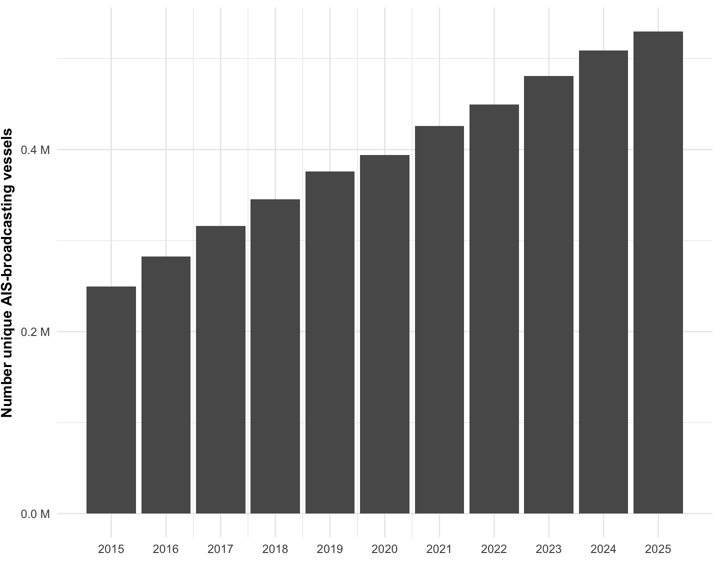
First, we look at total global number of active vessels per year from 2017 to 2025 (Figure 1.10, Table 1.7).
| vessel_class | 2015 | 2016 | 2017 | 2018 | 2019 | 2020 | 2021 | 2022 | 2023 | 2024 | 2025 |
|---|---|---|---|---|---|---|---|---|---|---|---|
| passenger | 70,173 | 84,334 | 100,688 | 117,307 | 133,761 | 141,807 | 164,357 | 182,248 | 198,621 | 217,474 | 232,497 |
| trawlers | 45,978 | 52,264 | 58,154 | 63,972 | 66,983 | 68,484 | 71,952 | 74,410 | 80,058 | 80,861 | 82,028 |
| cargo.general | 41,733 | 46,885 | 50,225 | 51,326 | 55,639 | 58,276 | 57,288 | 54,607 | 55,040 | 55,952 | 55,481 |
| tug | 25,778 | 28,062 | 31,053 | 32,386 | 35,324 | 37,229 | 38,546 | 38,833 | 40,463 | 43,041 | 44,460 |
| cargo.bulk_carrier | 11,972 | 12,670 | 13,107 | 13,189 | 13,688 | 14,206 | 14,899 | 15,523 | 16,040 | 16,806 | 17,130 |
| driftnets | 7,927 | 9,356 | 10,398 | 11,552 | 12,347 | 12,634 | 13,600 | 14,746 | 16,518 | 16,458 | 16,415 |
| tanker.oil | 9,989 | 10,202 | 10,583 | 11,091 | 11,191 | 11,315 | 11,517 | 11,824 | 11,972 | 12,769 | 13,499 |
| drifting_longlines | 3,104 | 3,838 | 4,646 | 5,238 | 5,874 | 6,657 | 8,284 | 10,012 | 10,806 | 11,421 | 11,919 |
| cargo.container | 5,098 | 5,141 | 5,322 | 5,315 | 5,410 | 5,461 | 5,803 | 5,931 | 6,338 | 6,855 | 7,220 |
| tanker.chemical | 4,730 | 4,928 | 5,100 | 5,243 | 5,430 | 5,469 | 5,632 | 5,852 | 5,954 | 6,138 | 6,529 |
| set_gillnets | 2,291 | 2,761 | 3,246 | 3,701 | 3,991 | 4,276 | 4,773 | 4,845 | 5,486 | 5,913 | 6,485 |
| supply_vessel | 4,290 | 4,086 | 3,929 | 3,991 | 4,092 | 4,052 | 4,039 | 4,255 | 4,403 | 4,556 | 4,587 |
| patrol_vessel | 2,273 | 2,470 | 2,759 | 3,026 | 3,140 | 3,315 | 3,515 | 3,852 | 4,162 | 4,389 | 4,565 |
| cargo.ro_ro | 2,387 | 2,505 | 2,601 | 2,747 | 3,009 | 3,089 | 3,215 | 3,514 | 3,732 | 4,051 | 4,300 |
| bunker | 1,837 | 2,121 | 2,322 | 2,437 | 2,665 | 2,776 | 2,605 | 2,539 | 3,543 | 3,780 | 3,834 |
| squid_jigger | 608 | 684 | 754 | 865 | 1,009 | 1,873 | 2,321 | 2,591 | 2,791 | 2,989 | 3,016 |
| dredge_non_fishing | 1,819 | 1,969 | 2,197 | 2,292 | 2,309 | 2,384 | 2,453 | 2,506 | 2,628 | 2,712 | 2,857 |
| pots_and_traps | 1,102 | 1,363 | 1,630 | 1,865 | 2,020 | 2,116 | 2,187 | 2,206 | 2,235 | 2,256 | 2,293 |
| tanker.liquefied_gas | 1,310 | 1,379 | 1,460 | 1,560 | 1,589 | 1,664 | 1,773 | 1,843 | 1,876 | 2,043 | 2,162 |
| other_not_fishing | 1,088 | 1,072 | 1,105 | 1,131 | 1,192 | 1,252 | 1,369 | 1,438 | 1,539 | 1,627 | 1,645 |
| pole_and_line | 451 | 539 | 614 | 697 | 758 | 842 | 968 | 1,058 | 1,188 | 1,308 | 1,372 |
| seismic_vessel | 1,086 | 1,096 | 1,086 | 1,114 | 1,121 | 1,121 | 1,130 | 1,155 | 1,229 | 1,249 | 1,293 |
| set_longlines | 423 | 448 | 471 | 492 | 545 | 597 | 655 | 712 | 763 | 811 | 816 |
| other_fishing | 8 | 5 | 17 | 38 | 46 | 118 | 232 | 371 | 501 | 629 | 714 |
| tuna_purse_seines | 424 | 514 | 549 | 569 | 621 | 641 | 660 | 678 | 669 | 671 | 674 |
| specialized_reefer | 518 | 516 | 530 | 531 | 530 | 504 | 499 | 479 | 471 | 463 | 447 |
| dive_vessel | 323 | 354 | 349 | 365 | 375 | 366 | 370 | 366 | 368 | 363 | 348 |
| trollers | 150 | 181 | 211 | 243 | 276 | 285 | 293 | 304 | 308 | 302 | 309 |
| dredge_fishing | 237 | 249 | 245 | 240 | 243 | 259 | 249 | 252 | 250 | 265 | 258 |
| other_seines | 154 | 160 | 168 | 171 | 175 | 174 | 180 | 176 | 177 | 173 | 171 |
| other_purse_seines | 82 | 85 | 91 | 93 | 96 | 101 | 111 | 109 | 115 | 124 | 125 |
| cargo.refrigerated | 136 | 161 | 192 | 207 | 202 | 189 | 178 | 141 | 128 | 122 | 120 |
| well_boat | 71 | 79 | 84 | 91 | 91 | 94 | 96 | 100 | 98 | 98 | 97 |
| container_reefer | 105 | 102 | 104 | 104 | 98 | 93 | 91 | 88 | 85 | 81 | 79 |
| research | 46 | 52 | 55 | 59 | 63 | 60 | 63 | 63 | 63 | 65 | 68 |
| tanker.other | 30 | 29 | 27 | 28 | 30 | 30 | 29 | 31 | 32 | 33 | 35 |
| fish_factory | 1 | 1 | 1 | 1 | 1 | 1 | 1 | 1 | 1 | 1 | NA |
1.2.1.2 Voyages
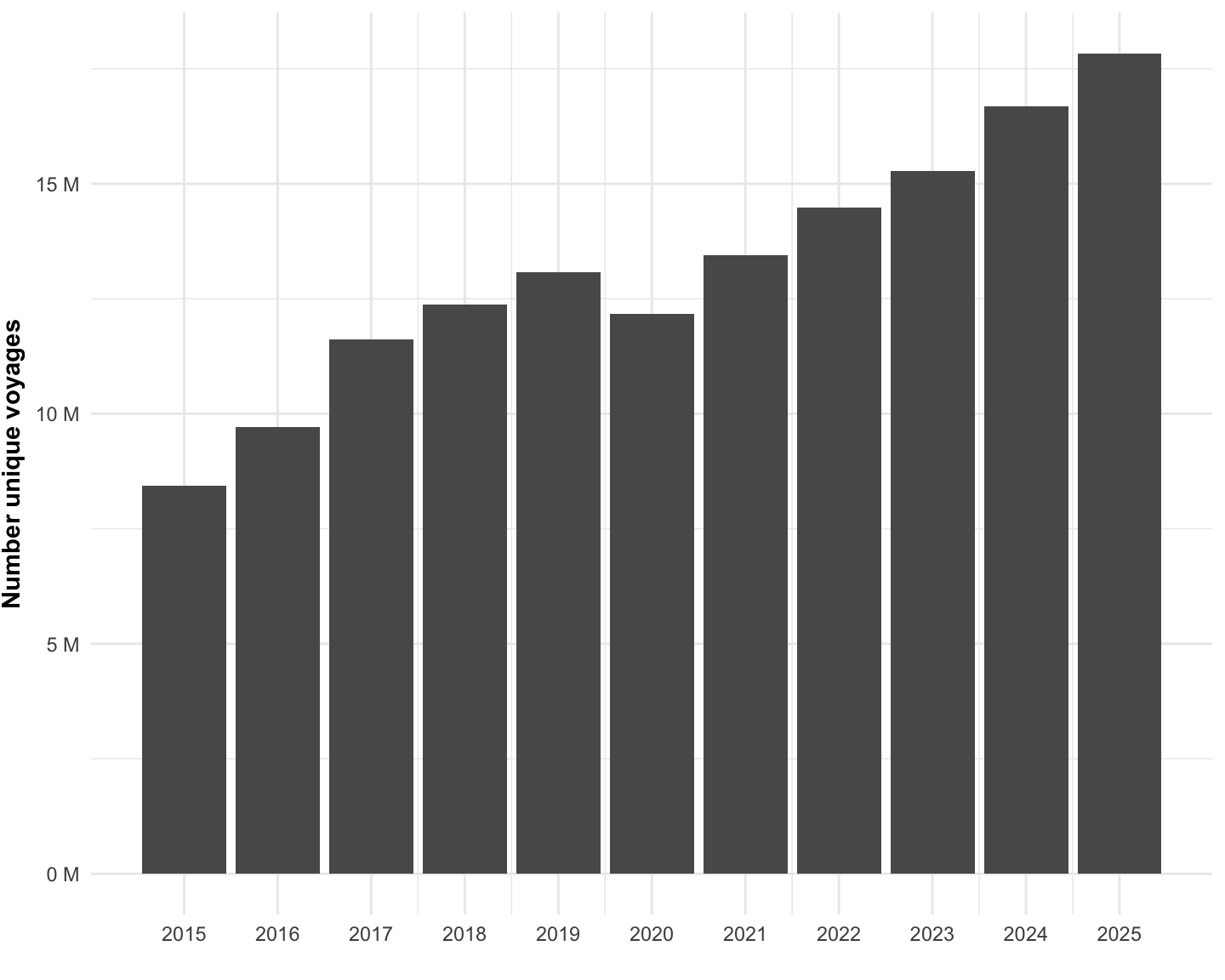
Next, we summarize the number of voyages, globally, for vessels included in our analysis from 2017 to 2025 (Figure 1.11, Table 1.8).
| year | n_unique_events |
|---|---|
| 2015 | 8,438,280 |
| 2016 | 9,703,995 |
| 2017 | 11,618,792 |
| 2018 | 12,366,760 |
| 2019 | 13,077,321 |
| 2020 | 12,168,457 |
| 2021 | 13,443,618 |
| 2022 | 14,488,865 |
| 2023 | 15,269,684 |
| 2024 | 16,690,511 |
| 2025 | 17,832,363 |
1.2.1.3 Port visits
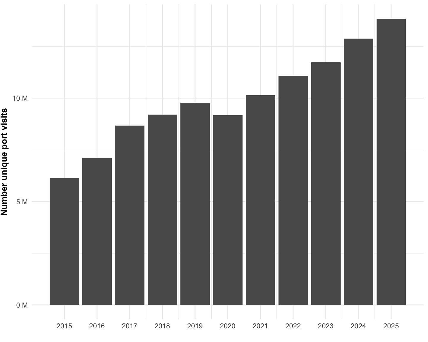
Here we summarize the time series trend of the number of port visits, globally, for the vessels included in our analysis from 2017 to 2025 (Figure 1.12, Table 1.9).
| year | n_unique_events |
|---|---|
| 2015 | 6,130,307 |
| 2016 | 7,124,252 |
| 2017 | 8,668,002 |
| 2018 | 9,198,674 |
| 2019 | 9,779,229 |
| 2020 | 9,175,171 |
| 2021 | 10,136,402 |
| 2022 | 11,078,046 |
| 2023 | 11,726,290 |
| 2024 | 12,880,422 |
| 2025 | 13,841,478 |
1.2.1.4 Emissions
Next, we look at total annual global emissions (metric tonnes, MT) for each pollutant from 2017 to 2025 (Figure 1.13, Table 1.10).
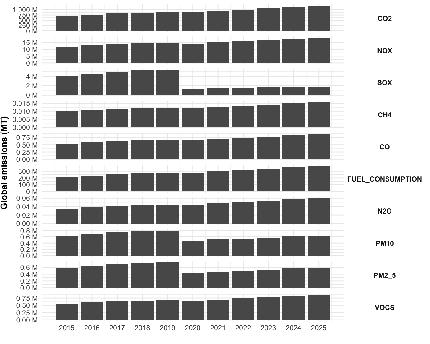
| year | CO2 | NOX | SOX | CH4 | CO | FUEL_CONSUMPTION | N2O | PM10 | PM2_5 | VOCS |
|---|---|---|---|---|---|---|---|---|---|---|
| 2015 | 687,187,536 | 12,093,759 | 4,180,377 | 9,797 | 534,100 | 216,494,170 | 34,915 | 640,827 | 589,561 | 552,161 |
| 2016 | 752,723,804 | 13,095,485 | 4,584,913 | 10,620 | 579,962 | 237,141,062 | 38,228 | 699,654 | 643,681 | 596,068 |
| 2017 | 824,218,655 | 14,107,633 | 5,025,029 | 11,473 | 627,651 | 259,665,170 | 41,785 | 761,982 | 701,023 | 640,725 |
| 2018 | 861,417,974 | 14,503,805 | 5,247,862 | 11,845 | 648,872 | 271,384,574 | 43,550 | 791,224 | 727,926 | 660,289 |
| 2019 | 884,081,785 | 14,601,273 | 5,389,357 | 12,030 | 659,256 | 278,524,749 | 44,566 | 807,368 | 742,779 | 668,481 |
| 2020 | 879,054,702 | 14,277,525 | 1,344,155 | 11,823 | 648,498 | 276,941,106 | 44,247 | 480,261 | 441,841 | 655,818 |
| 2021 | 941,098,607 | 15,219,708 | 1,440,008 | 12,594 | 691,790 | 296,487,859 | 47,391 | 513,630 | 472,539 | 699,712 |
| 2022 | 1,004,524,398 | 16,021,251 | 1,539,676 | 13,383 | 735,331 | 316,470,057 | 50,428 | 545,481 | 501,843 | 742,249 |
| 2023 | 1,054,249,167 | 16,739,653 | 1,617,398 | 14,150 | 775,723 | 332,135,589 | 52,905 | 573,653 | 527,761 | 781,788 |
| 2024 | 1,139,197,974 | 17,866,397 | 1,749,804 | 15,131 | 830,746 | 358,898,539 | 57,062 | 615,808 | 566,544 | 834,948 |
| 2025 | 1,189,412,753 | 18,473,718 | 1,829,501 | 15,760 | 864,984 | 374,718,694 | 59,523 | 640,958 | 589,681 | 867,643 |
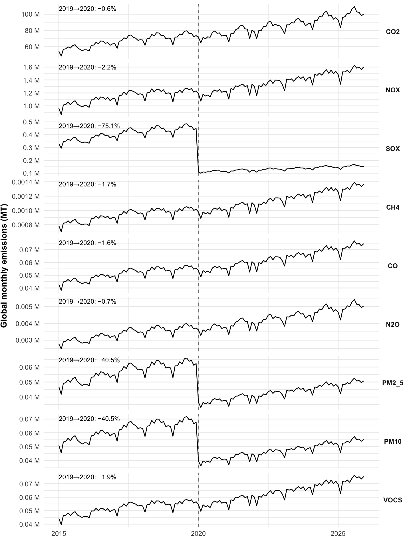
1.2.1.5 Monthly emissions time series
We can also examine the monthly time series of global emissions for each pollutant (Figure 1.14). The dashed vertical line marks January 2020, when the IMO 2020 low-sulfur fuel regulation took effect (capping marine fuel sulfur content at 0.5% outside Emission Control Areas). This regulation was designed to sharply reduce sulfur oxide (SOX) and particulate matter (PM) emissions; each facet is annotated with the change in annual emissions from 2019 to 2020 for that pollutant.
1.2.2 Emissions by vessel class
Next, for2025, we summarize the global annual emissions by vessel class (Figure 1.15). These are summarized using the GFW vessel class categories. We first plot simply CO2 emissions, then look at a table of all pollutants.
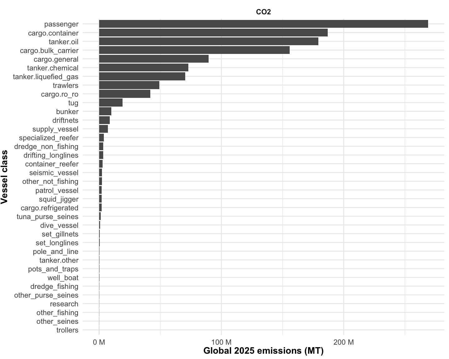
We next can look at a table of all pollutants for 2025 (Table 1.11):
| vessel_class | CO2 | NOX | SOX | FUEL_CONSUMPTION | VOCS | CO | PM10 | PM2_5 | N2O | CH4 |
|---|---|---|---|---|---|---|---|---|---|---|
| passenger | 268,857,697 | 1,893,746 | 416,396 | 84,703,502 | 87,747 | 114,840 | 92,660 | 85,247 | 12,268 | 1,862 |
| cargo.container | 186,915,291 | 4,214,199 | 289,631 | 58,886,883 | 203,817 | 179,159 | 127,519 | 117,318 | 9,883 | 3,425 |
| tanker.oil | 179,115,998 | 2,244,436 | 276,422 | 56,429,934 | 104,680 | 106,678 | 82,930 | 76,296 | 8,654 | 1,858 |
| cargo.bulk_carrier | 155,827,619 | 3,427,372 | 241,496 | 49,092,943 | 159,817 | 142,445 | 104,664 | 96,291 | 8,179 | 2,655 |
| cargo.general | 89,617,662 | 1,426,469 | 138,676 | 28,233,215 | 67,744 | 74,267 | 52,978 | 48,740 | 4,679 | 1,389 |
| tanker.chemical | 72,973,721 | 1,113,333 | 113,089 | 22,990,095 | 51,224 | 51,165 | 38,747 | 35,647 | 3,653 | 916 |
| tanker.liquefied_gas | 70,418,534 | 1,185,784 | 97,786 | 22,183,852 | 53,624 | 51,451 | 38,831 | 35,725 | 3,624 | 907 |
| trawlers | 49,380,063 | 919,413 | 76,481 | 15,556,830 | 40,896 | 44,153 | 31,426 | 28,912 | 2,523 | 818 |
| cargo.ro_ro | 41,832,972 | 870,535 | 64,621 | 13,179,229 | 38,808 | 37,268 | 27,157 | 24,984 | 2,207 | 693 |
| tug | 19,118,142 | 334,974 | 29,620 | 6,023,071 | 19,669 | 19,668 | 12,853 | 11,825 | 1,042 | 412 |
| bunker | 9,971,218 | 59,039 | 15,457 | 3,141,413 | 2,596 | 3,692 | 3,117 | 2,868 | 450 | 57 |
| driftnets | 8,845,856 | 152,282 | 13,693 | 2,786,792 | 6,668 | 7,596 | 5,399 | 4,967 | 445 | 141 |
| supply_vessel | 7,154,271 | 110,345 | 11,070 | 2,253,862 | 6,586 | 6,999 | 4,674 | 4,300 | 385 | 140 |
| specialized_reefer | 3,825,616 | 62,999 | 5,922 | 1,205,221 | 2,624 | 3,099 | 2,226 | 2,048 | 201 | 57 |
| dredge_non_fishing | 3,431,583 | 61,475 | 5,315 | 1,081,096 | 3,005 | 3,267 | 2,247 | 2,067 | 185 | 64 |
| drifting_longlines | 3,293,071 | 62,599 | 5,104 | 1,037,470 | 2,570 | 2,803 | 1,985 | 1,826 | 163 | 52 |
| container_reefer | 2,751,094 | 67,703 | 4,261 | 866,711 | 2,520 | 2,539 | 1,837 | 1,690 | 149 | 47 |
| seismic_vessel | 2,467,237 | 42,923 | 3,797 | 777,279 | 2,648 | 2,552 | 1,694 | 1,558 | 135 | 54 |
| other_not_fishing | 2,354,982 | 31,960 | 3,511 | 741,905 | 1,428 | 1,664 | 1,194 | 1,099 | 121 | 31 |
| patrol_vessel | 2,158,613 | 32,166 | 3,060 | 680,020 | 1,820 | 1,905 | 1,298 | 1,194 | 118 | 37 |
| squid_jigger | 2,080,631 | 34,644 | 3,221 | 655,483 | 1,642 | 1,794 | 1,283 | 1,180 | 104 | 33 |
| cargo.refrigerated | 2,064,960 | 41,576 | 3,191 | 650,546 | 1,728 | 1,835 | 1,322 | 1,216 | 111 | 34 |
| tuna_purse_seines | 1,353,763 | 23,858 | 2,096 | 426,492 | 1,075 | 1,155 | 825 | 759 | 66 | 21 |
| dive_vessel | 853,406 | 12,963 | 1,321 | 268,855 | 756 | 810 | 554 | 509 | 45 | 16 |
| set_gillnets | 630,227 | 11,157 | 977 | 198,552 | 472 | 520 | 365 | 336 | 30 | 10 |
| set_longlines | 457,897 | 8,133 | 710 | 144,259 | 347 | 386 | 272 | 250 | 22 | 7 |
| pole_and_line | 360,850 | 6,665 | 559 | 113,685 | 272 | 300 | 211 | 194 | 17 | 6 |
| tanker.other | 285,844 | 2,026 | 444 | 90,056 | 82 | 113 | 93 | 86 | 13 | 2 |
| pots_and_traps | 229,351 | 4,348 | 356 | 72,258 | 170 | 185 | 129 | 118 | 11 | 3 |
| well_boat | 211,020 | 3,520 | 327 | 66,480 | 173 | 192 | 134 | 123 | 11 | 4 |
| dredge_fishing | 167,306 | 3,427 | 260 | 52,714 | 124 | 139 | 96 | 88 | 8 | 3 |
| other_purse_seines | 138,976 | 2,899 | 216 | 43,785 | 106 | 117 | 81 | 75 | 7 | 2 |
| research | 87,670 | 1,645 | 136 | 27,621 | 73 | 82 | 56 | 52 | 5 | 2 |
| other_fishing | 80,875 | 1,186 | 125 | 25,479 | 61 | 66 | 46 | 42 | 4 | 1 |
| other_seines | 58,399 | 1,144 | 91 | 18,399 | 43 | 47 | 33 | 30 | 3 | 1 |
| trollers | 40,337 | 775 | 63 | 12,709 | 29 | 31 | 21 | 19 | 2 | 1 |
1.2.3 Spatial maps of emissions
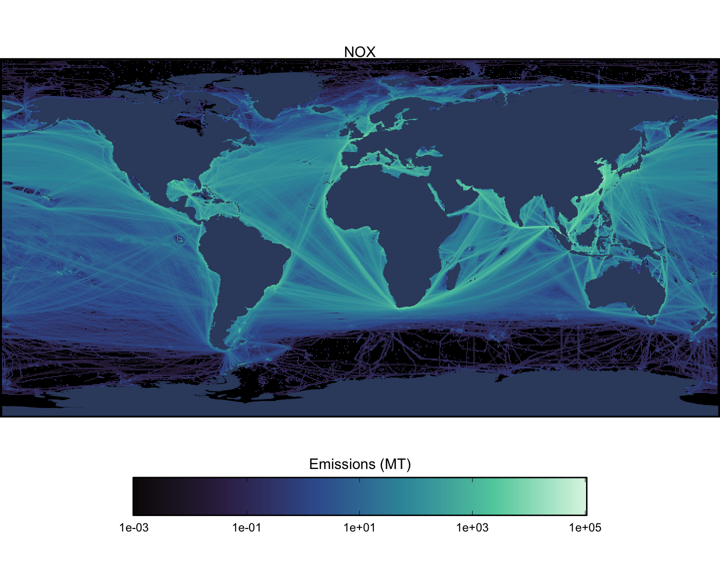
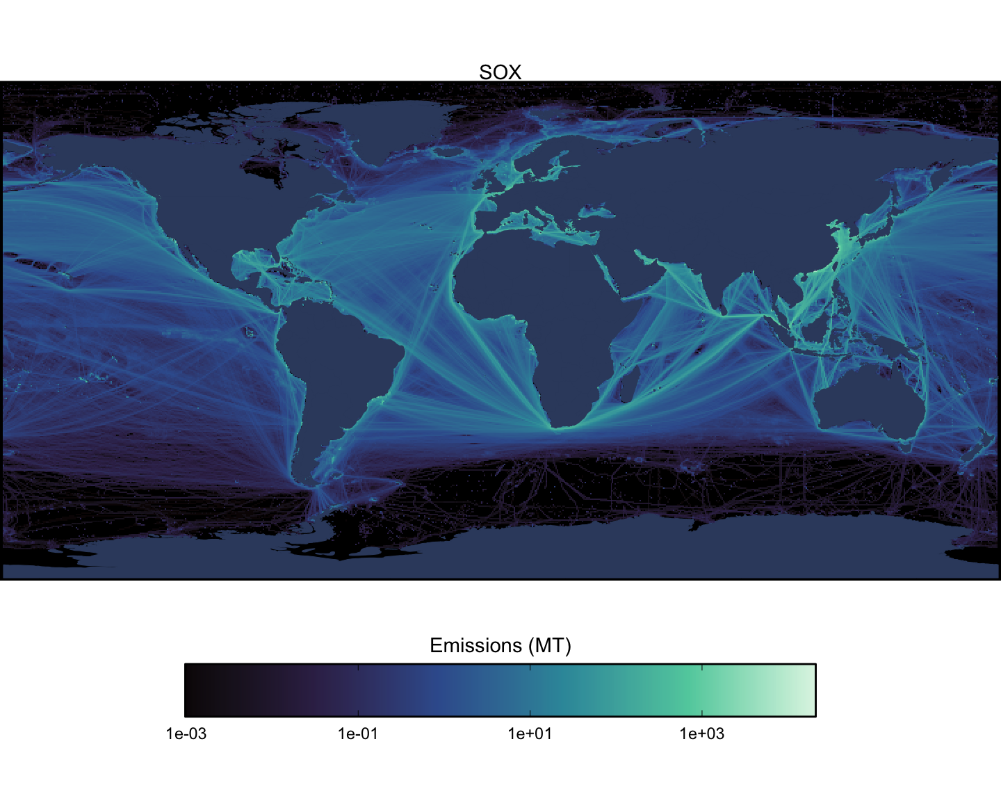
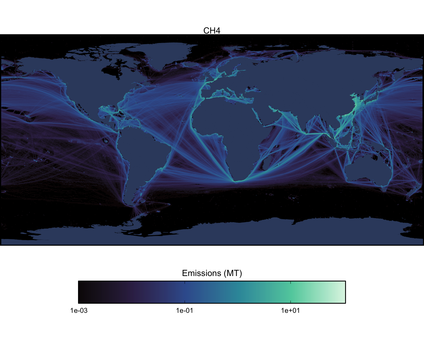
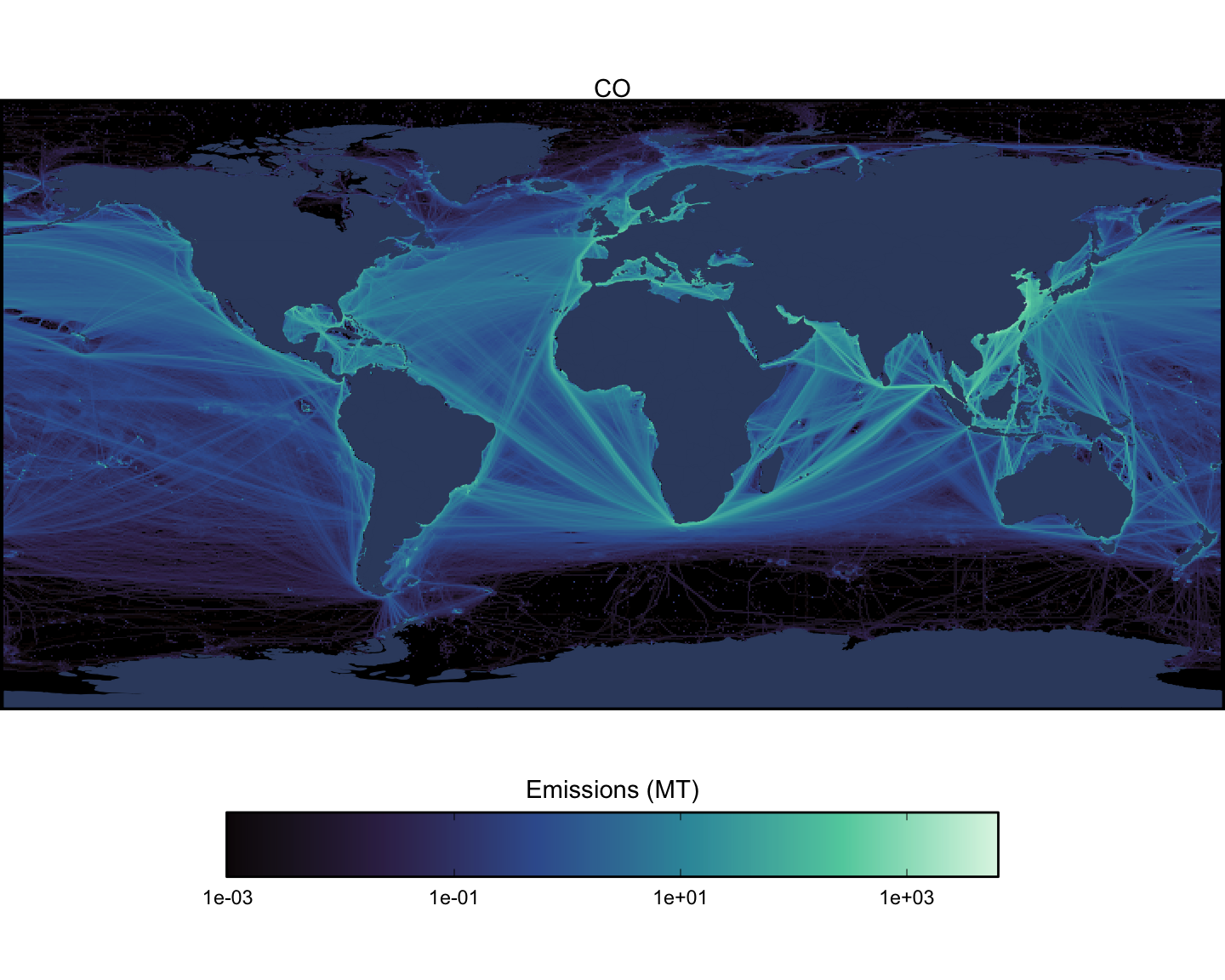
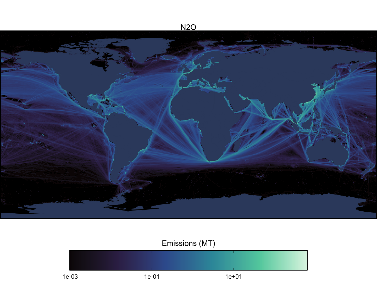
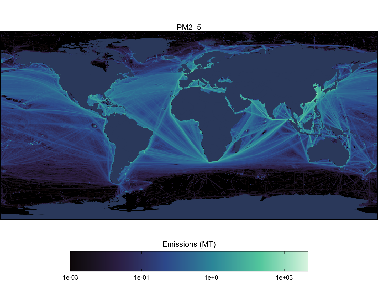
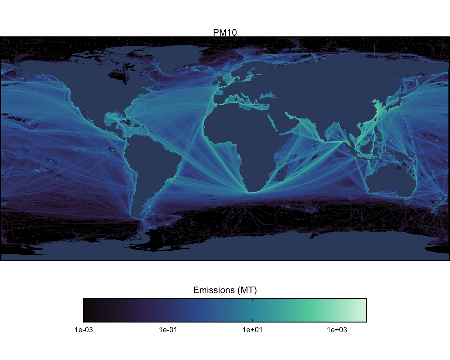
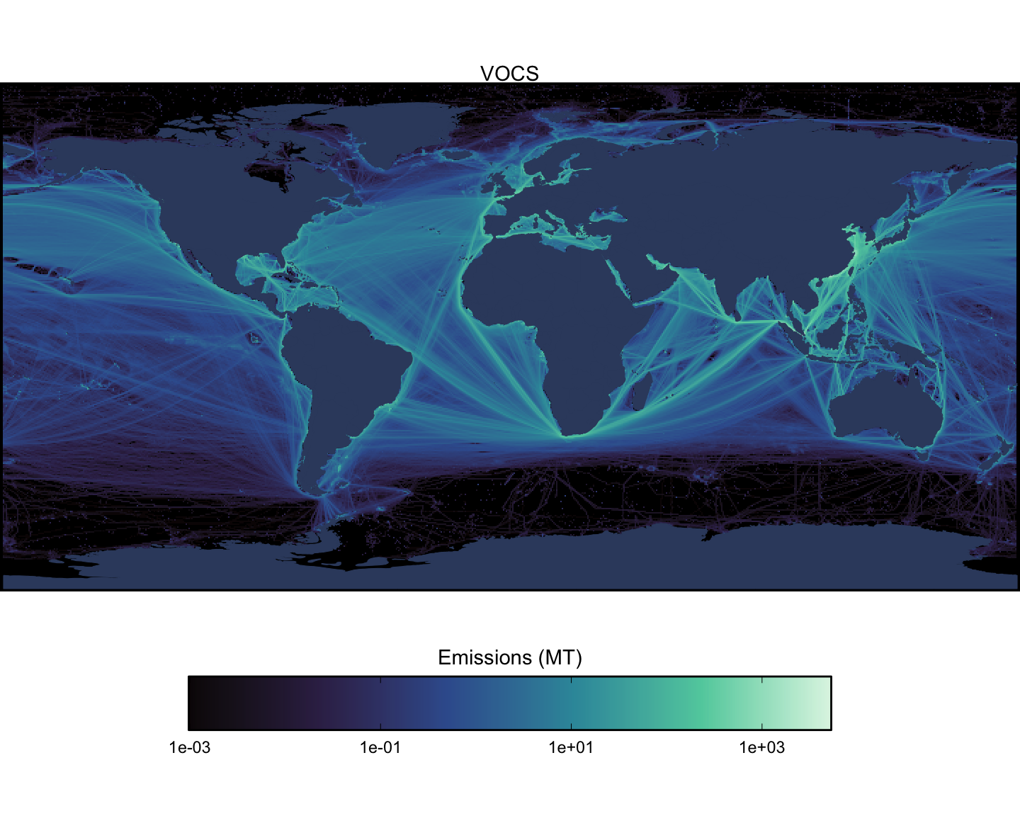
Next we can look at spatial maps of emissions by pollutant, aggregated across all vessel types. These maps are shown at a spatial resolution of 0.1x0.1 degrees (Figure 1.16 - Figure 1.24).
Reading layer `World_Countries_Generalized' from data source
  `/Users/gmcdonald/github/ocean-ghg/data/raw/World_Countries_Generalized_Shapefile/World_Countries_Generalized.shp'
  using driver `ESRI Shapefile'
Simple feature collection with 251 features and 4 fields
Geometry type: MULTIPOLYGON
Dimension:     XY
Bounding box:  xmin: -20037510 ymin: -30240970 xmax: 20037510 ymax: 18418390
Projected CRS: WGS 84 / Pseudo-Mercator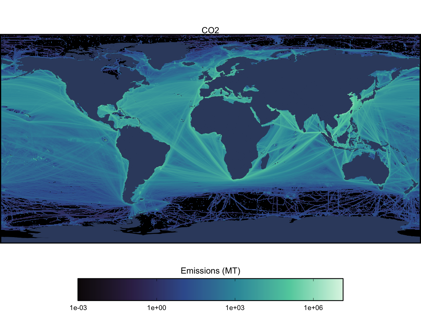
1.3 Model Validation
The initial stages of model development involved multiple rounds of preliminary validation against testing model versions to identify the best-performing one among those evaluated. Following this testing phase, and with the AIS-based model built as described above, we validated it against measured absolute emission values from a dataset of a European Union (EU) monitoring program.
1.3.1 EU emissions data
We used the \(CO_2\) emissions data from maritime transport provided by the European Maritime Safety Agency, which is part of the monitoring, reporting, and verification program of carbon emissions from maritime transport, set by the Regulation (EU) 2015/757. As detailed below, vessels with certain characteristics and certain trips made by such vessels operating in EEA sea ports, must report their emissions on an annual basis.
1.3.1.1 What’s in an out of EU 2015/757
Here, we summarize the relevant provisions of this legislation that define the vessels and trip characteristics that need to be filtered from our data for validation purposes.
Vessel characteristics:
Ships above 5000 gross tonnage.
Excludes warships, naval auxiliaries, fish-catching or fish-processing ships, wooden ships of a primitive build, ships not propelled by mechanical means, or government ships used for non-commercial purposes.
Trips characteristics:
Trips from their last port of call to a port of call under the jurisdiction of a Member State and from a port of call under the jurisdiction of a Member State to their next port of call, as well as within ports of call under the jurisdiction of a Member State.
Vessel activities covered by the law are those when the ships are at sea as well as at berth.
Ship at berth includes any ship which is securely moored or anchored in a port falling under the jurisdiction of a Member State while it is loading, unloading or hotelling, including the time spent when not engaged in cargo operations.
Port of call means the port where a ship stops to load or unload cargo or to embark or disembark passengers; consequently, stops for the sole purposes of refueling, obtaining supplies, relieving the crew, going into dry-dock or making repairs to the ship and/or its equipment, stops in port because the ship is in need of assistance or in distress, ship-to-ship transfers carried out outside ports, and stops for the sole purpose of taking shelter from adverse weather or rendered necessary by search and rescue activities are excluded.
Ship to ship transfers carried out outside ports are covered by the Regulation when these transfers take place as part of a voyage starting and/or ending with a port of call under the jurisdiction of a Member State.
A ship to ship transfer carried out outside ports is not considered as a port of call. As a consequence, if for example, a vessel leaves an EEA port, arrives to a US harbor performs a ship to ship operation outside the port limits, and then goes to South Corea the emissions falling within MRV scope will be the emissions released during the whole voyage from the EEA port of call until the port of call in South Korea. However, if the ship to ship transfer can be carried out within the port limits, that operation would constitute a port of call. The voyage covered by the MRV Maritime Regulation would then be an EEA port of call to a US port of call.
If a ship performs more than 300 voyages during the reporting period and all of these voyages either start from or end in a port within a Member State, the company can be exempted from monitoring the detailed parameters for each voyage.
Time ranges:
- The reporting period covers one calendar year during which CO2 emissions have to be monitored. For voyages starting and ending in two different calendar years, the monitoring and reporting data shall be accounted under the first calendar year concerned.
1.3.2 Data filtering
Given the law’s exceptions, in order to validate emission estimates, we need to filter our results to match the EU data contents and aggregation. In this regard, the vessel characteristics in terms of type and gross tonnage can be filtered by simply assessing which vessel IDs are included in the EU dataset. As for the time range, since the data is aggregated yearly by the starting date of a trip, the filtering is straightforward.
The most challenging aspect of this data filtering corresponds to the trip characteristics, specifically when defining the “ports of call.” The main obstacle is the inability to determine the type of activity a vessel is engaged in while in port, which prevents us from identifying which trips are included within those aggregated yearly emissions. To work around this, and establish which vessels’ emissions can be included in the validation, we have compared the total distance and total hours at sea reported in the EU data to the total distance traveled across all trips in our trip-level emissions for that vessel and year. If these numbers were within ±5%, ±10%, or ±15% difference, then we could reasonably assumed that aggregated trips in the GFW dataset correspond to trips included in the EU dataset.
The EU data has been compiled and stored in proj_ocean_ghg.eu_validation_data, while the selection and part of the filtering from our data has been conducted through the queries in eu_validation_trip.sql and eu_validation_port.sql, differentiating between emissions by trip and port visits, and stored in proj_ocean_ghg.eu_validation_trip and proj_ocean_ghg.eu_validation_port respectively.
1.3.3 Validation results
Emissions estimates are divided between emissions at sea and emissions at port. Here, we present the differences between our results and the EU emissions data.
1.3.3.1 Trip emissions
As detailed in the Methods section, we have defined trip emissions as those occurring between ports. In the EU dataset, these emissions are categorized under three variables: emissions from EEA-EEA, EEA-NonEEA, and NonEEA-EEA seaports. We have run our model, selected the data by trips involving at least one EEA port, aggregated the results by year, and selected vessels listed in the EU dataset for a specific year.
After discarding 1063 observations with no time at sea, and assessing potential duplicates due to different ssvid for the same imo_number (0 duplicates in this dataset), we ended up with a total of 212525 observations—year and vessel—selected from our emission estimates. This is 86.4% of the EU data observations. By applying different margin values to the annual hours at sea we get the following performance metrics detailed in Table 1.12. As we can see, higher performance is achieved applying a 10% margin, with which we obtained a selection of 20432 observations for validation.
| mae | rmse | nrmse | rsq | rsq_trad | mape | mpe | threshold | n_observations |
|---|---|---|---|---|---|---|---|---|
| 2290.683 | 5074.885 | 0.414 | 0.840 | 0.829 | Inf | -Inf | 0.05 | 11621 |
| 2492.546 | 5277.990 | 0.397 | 0.855 | 0.843 | Inf | -Inf | 0.10 | 20432 |
| 2578.680 | 5409.534 | 0.403 | 0.852 | 0.838 | Inf | -Inf | 0.15 | 27657 |
| 2608.295 | 5401.652 | 0.409 | 0.849 | 0.832 | Inf | -Inf | 0.20 | 33753 |
| 2650.764 | 5506.945 | 0.423 | 0.839 | 0.821 | Inf | -Inf | 0.25 | 38980 |
| 2701.098 | 5545.511 | 0.432 | 0.833 | 0.813 | Inf | -Inf | 0.30 | 43958 |
| 2761.555 | 5619.797 | 0.442 | 0.826 | 0.804 | Inf | -Inf | 0.35 | 48399 |
| 2843.186 | 5770.170 | 0.456 | 0.816 | 0.792 | Inf | -Inf | 0.40 | 52490 |
Comparing against the EU dataset with that 10% margin, the model demonstrates a good fit with an R-squared value of 0.85. While the MAE and RMSE indicate a considerable average magnitude of prediction errors, we need to consider that the average emission values are quite large since we are estimating absolute emissions per year. In fact, the normalized RMSE suggests that the errors, relative to the range of observed values, are moderate. Further, the model exhibits a tendency to underestimate emissions, as evidenced by the MPE. Despite some limitations, this validation framework offers a useful alternative to the one derived from the ML results, avoiding the related outlier inconveniences from emissions expressed in distance units. We can visually explore the relationship between our results and the EU data, observing certain linearity between both emission values with some spreading as the emission values increase (Figure 1.25).
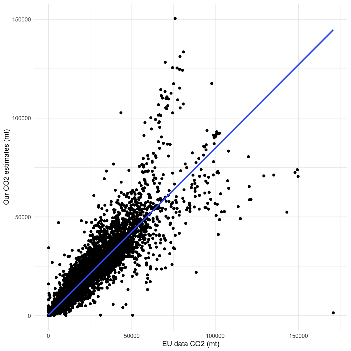
We can double-check these results by applying the data filtering margin on distance traveled instead of hours. In this regard, while the EU dataset does not contain information on the total nautical miles (nm) navigated, we can extract this from the annual average \(CO_2\) emissions per distance. If we apply distinct margins to the total nautical miles (nm) navigated, we achieve the highest performance values for the 25% margin, with which we select 44211 observations. Overall, the performance metrics are slightly worse than those obtained by using hours at sea, which was a direct measure available in the EU dataset, rather than an indirect estimate like total nm navigated (Figure 1.26 and Table 1.13).
| mae | rmse | nrmse | rsq | rsq_trad | mape | mpe | threshold | n_observations |
|---|---|---|---|---|---|---|---|---|
| 2483.654 | 5482.283 | 0.400 | 0.852 | 0.840 | Inf | -Inf | 0.05 | 18819 |
| 2586.578 | 5428.002 | 0.401 | 0.854 | 0.839 | Inf | -Inf | 0.10 | 27956 |
| 2644.225 | 5422.718 | 0.409 | 0.850 | 0.833 | Inf | -Inf | 0.15 | 34406 |
| 2696.778 | 5512.987 | 0.422 | 0.842 | 0.822 | Inf | -Inf | 0.20 | 39627 |
| 2736.045 | 5627.718 | 0.436 | 0.830 | 0.810 | Inf | -Inf | 0.25 | 44211 |
| 2764.120 | 5643.478 | 0.443 | 0.825 | 0.803 | Inf | -Inf | 0.30 | 48211 |
| 2809.374 | 5696.090 | 0.452 | 0.818 | 0.795 | Inf | -Inf | 0.35 | 52004 |
| 2874.533 | 5806.600 | 0.463 | 0.810 | 0.786 | Inf | -Inf | 0.40 | 55456 |
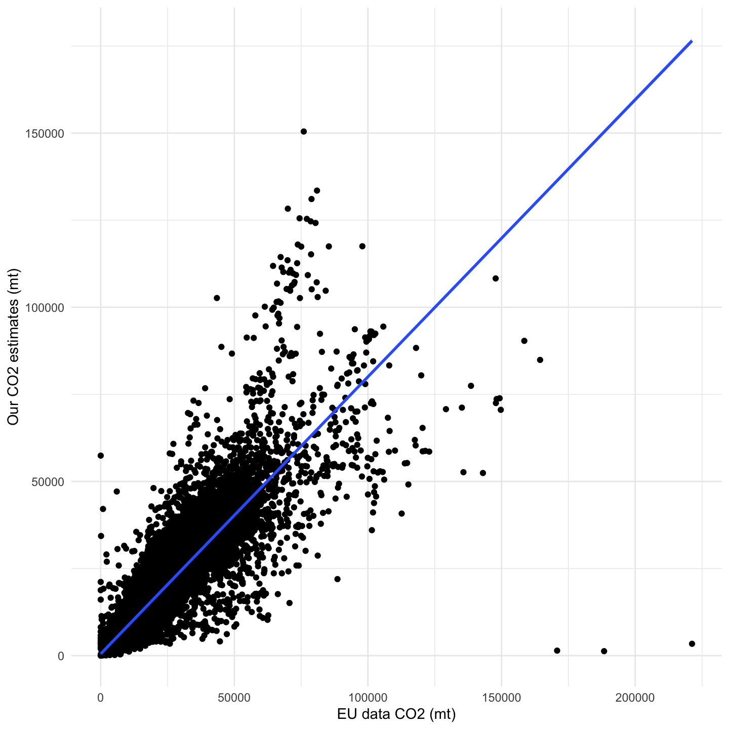
1.3.3.2 Port emissions
As for emissions at ports, these consist of emissions during port stays. Here, we have filtered those emission results by port visits within the EEA and followed the same aggregation procedure as for trips. However, some assumptions have been made due to the impossibility of filtering out stays that may not be included in the EU dataset. As mentioned earlier, one of the inconveniences related to using this dataset is the definition of “ports of call”, which establishes whether a vessel trip and port visit is considered or not under the regulation and, by extension, whether its emissions are reported and available in the EU dataset. Unable to define the activities performed by a vessel in a port, we assume that we will be overestimating the emissions at port since the EU does not include them all. With it, and applying the same procedure, we see that the performance values are quite poor given that overestimation, leaving us with the need to find an alternative way to validate our port emission results while improving our models estimates (Table 1.14 and Figure 1.27).
| model | mae | rmse | nrmse | rsq | rsq_trad | mape | mpe |
|---|---|---|---|---|---|---|---|
| Model 6.3 | 997.798 | 2564.964 | 1.893 | 0.164 | -2.584 | Inf | -Inf |
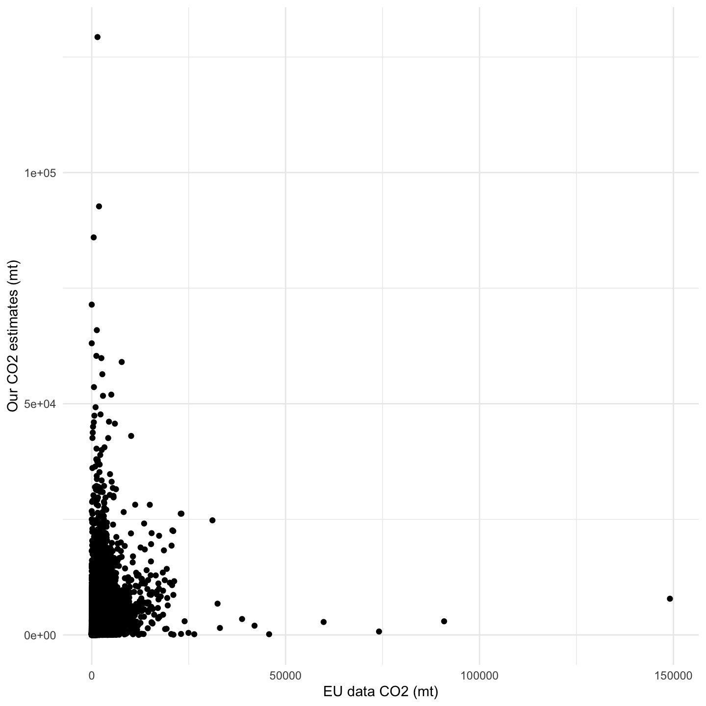
By applying an additional filtering step, selecting those observations from the trips under the 10% hours at sea margin approach, we would expect to narrow down our observations to those actually happening under “ports of call”. However, as the performance values in Table 1.15 and the emissions relationship shown in Figure 1.28 indicate, our model still does not capture emissions at port as reflected in the EU dataset, highlighting the need for improvement in this aspect.
| model | mae | rmse | nrmse | rsq | rsq_trad | mape | mpe |
|---|---|---|---|---|---|---|---|
| Model 6.3 | 961.368 | 2198.915 | 2.01 | 0.253 | -3.04 | Inf | -Inf |
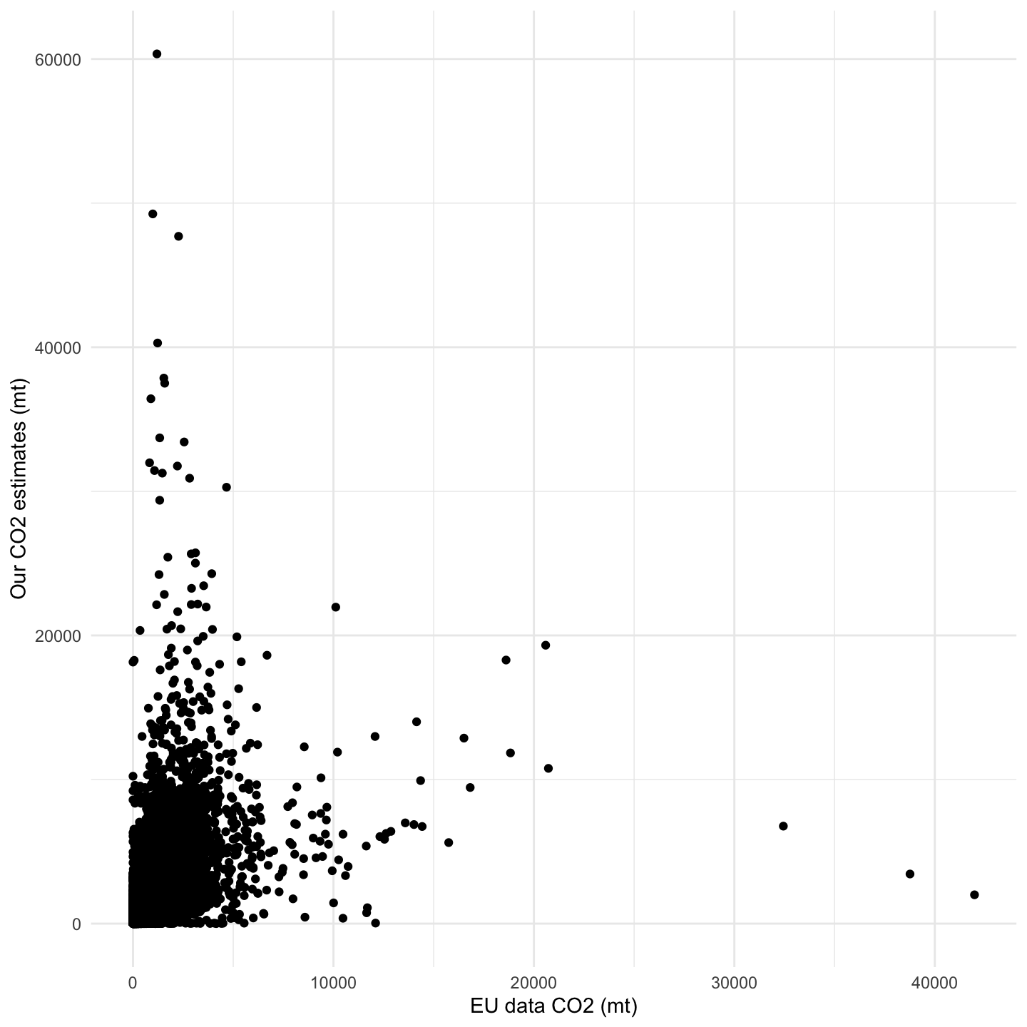
1.3.4 Comparison to other global emissions estimates
Several other emissions estimates have been done by the International Maritime Organization (IMO) (most recently for 2018), Emissions Database for Global Atmospheric Research (EDGAR) in (most recently for 2024), Organization for Economic Co-operation and Development (OECD) (most recently for 2024 using their experimental database). Below we compare our GHG emissions estimates with the findings of these studies to validate our results
The emissions inventories used in this comparison rely on a range of methods and have some differences in sector definitions and underlying data sources. Here we compare the most recent year of data from each inventory.
Highlights include:
GFW’s total estimated emissions (1.48 billion MT CO2 for both AIS-broadcasting vessels and dark vessels, and 1.14 billion MT CO2 for just AIS-broadcasting vessels) are similar to OECD, EDGAR, and IMO, indicating high reliability and utility of our methodology and results.
IMO’s, OECD’s, and EDGAR’s emissions estimates do not include dark fleets, making GFW’s dark fleet estimates the first of their kind.
| CO2 emissions (billion MT) | Data source |
|---|---|
| 1.48 | GFW (2024, AIS + S1) |
| 1.14 | GFW (2024, AIS) |
| 0.97 | OECD (2024) |
| 0.89 | EDGAR (2024) |
| 1.06 | IMO (2018) |
1.4 Available data tables (BigQuery)
This section documents the main result tables produced by the AIS-based emissions model so that we and other researchers know what data are available to work with. All tables live in the proj_ocean_ghg BigQuery dataset and carry a model-version suffix (currently _v20260714), so a table name looks like proj_ocean_ghg.vessel_info_v20260714. The delivered Climate TRACE product built from these tables is described separately in Chapter 3.
The tables share a small set of join keys: ssvid (the AIS Maritime Mobile Service Identity / MMSI, the vessel identifier), trip_id (a voyage), and visit_id (a port visit). Unless noted otherwise, all emissions columns are in metric tonnes (mt), energy-use columns are in kilowatt-hours (kWh), and the nine modeled pollutants are CO₂, CH₄, N₂O, NOₓ, SOₓ, CO, VOCs (NMVOC), PM2.5, and PM10. fuel_consumption_mt is an internal validation output and is not part of the delivered Climate TRACE schema (see Section 1.1.6).
1.4.1 vessel_info — vessel characteristics
The master vessel reference table. One row per vessel (ssvid). Holds identity, dimensions, and engine specifications, and is the source of the vessel metadata that drives the emissions calculation. Includes only vessels with a usable (non-gear) vessel-class prediction and without offsetting/overlapping-identity problems.
| Column | Description |
|---|---|
ssvid |
Vessel identifier (MMSI). |
flag |
Best flag state (ISO3) for the vessel. |
registries_listed |
Semicolon-separated list of registries the vessel appears in. |
ship_name_registry / ship_name_ais |
Best-known ship name from registries / from AIS broadcasts. |
callsign_registry / callsign_ais |
Best-known callsign from registries / from AIS. |
imo_registry / imo_ais |
Best-known IMO number from registries / from AIS. |
vessel_class |
Highest-resolution GFW vessel class available for the vessel. |
vessel_class_characteristics_source |
Source table for the vessel-class and characteristic predictions. |
main_engine_power_kw |
Main engine power (kW). |
tonnage_gt |
Gross tonnage (GT). |
length_m |
Vessel length (m). |
design_speed_knots |
Design (maximum) speed (knots). |
engine_type |
Engine type (e.g. oil/reciprocating, gas, turbine). |
engine_rpm |
Engine RPM. |
year_of_build |
Vessel year of build. |
is_fishing_vessel_class |
Whether the vessel_class is a fishing class. |
avg_aux_boiler_power_{berth,anchored,maneuvering,sea}_kw |
Boiler power demand (kW) in each of the four operational phases (Table 17, small-vessel-corrected). |
avg_aux_engine_power_{berth,anchored,maneuvering,sea}_kw |
Auxiliary-engine power demand (kW) in each of the four operational phases. |
1.4.2 ping_level_emissions — per-message emissions
Emissions and energy use computed for every individual AIS message (ping) — one row per (ssvid, timestamp). This is the finest-grain output and the source from which every other AIS table is aggregated. ⚠️ This is an extremely large table (on the order of 10¹¹ rows). Most users should work with the aggregated tables below rather than querying this one directly; it is documented here for completeness and for special-purpose analyses.
| Column | Description |
|---|---|
ssvid |
Vessel identifier (MMSI). |
timestamp |
Timestamp of the AIS message. |
hours |
Hours elapsed since the previous message (time the ping represents). |
lat / lon |
Position of the message. |
distance_nm |
Distance travelled since the previous message (nautical miles). |
speed_knots |
Speed used in the model (AIS-broadcast speed for gaps ≤1 h, implied speed otherwise). |
fishing_activity |
Whether the vessel was actively fishing at this ping. |
receiver_type |
AIS receiver type (terrestrial vs satellite). |
operational_phase |
Assigned phase: at_berth, anchored, maneuvering, or at_sea. |
main_engine_load_factor |
Computed main-engine load factor for the ping. |
main_engine_energy_use_kwh |
Main-engine energy use (kWh). |
aux_engine_energy_use_kwh |
Auxiliary-engine energy use (kWh). |
aux_boiler_energy_use_kwh |
Boiler energy use (kWh). |
emissions_{co2,ch4,n2o,nox,sox,co,vocs,pm2_5,pm10}_mt |
Ping-level emissions of each pollutant (mt). |
fuel_consumption_mt |
Ping-level fuel consumption (mt); internal output, not in the CT schema. |
1.4.3 daily_gridded_emissions_by_vessel — gridded daily emissions
Ping-level emissions aggregated to one row per vessel × day × 0.1° grid cell, split by fishing activity. This is the primary spatially- and temporally-explicit analysis table.
| Column | Description |
|---|---|
ssvid |
Vessel identifier (MMSI). |
date |
Calendar date. |
fishing_activity |
Whether the vessel was fishing (rows are split by this). |
lon_bin / lat_bin |
Lower-left corner of the 0.1° grid cell. |
hours |
Total hours of activity in the cell on that day. |
distance_nm |
Total distance travelled (nautical miles). |
emissions_{co2,ch4,n2o,nox,sox,co,vocs,pm2_5,pm10}_mt |
Summed emissions of each pollutant (mt). |
fuel_consumption_mt |
Summed fuel consumption (mt). |
1.4.4 voyage_info + trip_level_emissions — voyage-level data
voyage_info identifies each voyage (one row per trip_id); trip_level_emissions holds the emissions and energy totals for that voyage. Join the two on trip_id. Voyages use GFW confidence-3+ anchorage-to-anchorage trips and exclude durations under 1 minute or over ~365 days.
voyage_info
| Column | Description |
|---|---|
ssvid |
Vessel identifier (MMSI). |
vessel_id |
GFW internal vessel-id (used to filter unreliable “ghost” identities). |
trip_id |
Voyage identifier. |
departure_timestamp / arrival_timestamp |
Start and end of the voyage. |
from_anchorage_id / to_anchorage_id |
Origin and destination anchorage (S2 cell) ids. |
from_port / to_port |
Origin and destination port names. |
from_country_iso3 / to_country_iso3 |
Origin and destination country (ISO3). |
trip_start_confidence / trip_end_confidence |
GFW voyage confidence levels (3 or 4). |
route_string_from_anchorage_to_anchorage_wkt |
WKT LINESTRING from origin to destination anchorage. |
trip_level_emissions
| Column | Description |
|---|---|
ssvid |
Vessel identifier (MMSI). |
trip_id |
Voyage identifier (join key to voyage_info). |
hours |
Total voyage hours. |
distance_nm |
Total voyage distance (nautical miles). |
emissions_{co2,ch4,n2o,nox,sox,co,vocs,pm2_5,pm10}_mt |
Total voyage emissions of each pollutant (mt). |
fuel_consumption_mt |
Total voyage fuel consumption (mt). |
main_engine_energy_use_kwh / aux_engine_energy_use_kwh / aux_boiler_energy_use_kwh |
Total energy use by engine (kWh). |
1.4.5 port_visit_info + port_visit_level_emissions — port-visit data
Analogous to the voyage tables, but for port stays. port_visit_info identifies each visit (one row per visit_id) and port_visit_level_emissions holds its emissions/energy totals; join on visit_id. Visits use GFW confidence-3+ port visits, require the same start and end port/country, and exclude durations under 1 minute or over ~365 days.
port_visit_info
| Column | Description |
|---|---|
ssvid |
Vessel identifier (MMSI). |
vessel_id |
GFW internal vessel-id. |
visit_id |
Port-visit identifier. |
start_timestamp / end_timestamp |
Start and end of the port visit. |
from_anchorage_id / to_anchorage_id |
Entry and exit anchorage (S2 cell) ids within the port. |
from_port / to_port |
Port name (equal by construction). |
from_country_iso3 / to_country_iso3 |
Port country ISO3 (equal by construction). |
confidence |
GFW port-visit confidence (3 or 4). |
route_string_from_anchorage_to_anchorage_wkt |
WKT LINESTRING between entry and exit anchorage. |
port_visit_level_emissions — identical column layout to trip_level_emissions, but keyed on visit_id instead of trip_id (ssvid, visit_id, hours, distance_nm, the nine emissions_*_mt, fuel_consumption_mt, and the three *_energy_use_kwh columns).
1.4.6 monthly_spatial_vessel_emissions_by_receiver_type — gridded monthly emissions by AIS source
Emissions aggregated to one row per vessel × month × 1° grid cell × AIS receiver type, used to assess how estimates vary between terrestrially- and satellite-received AIS. Note this table carries CO₂ only (plus fuel), not all nine pollutants.
| Column | Description |
|---|---|
ssvid |
Vessel identifier (MMSI). |
month |
Month (timestamp truncated to month). |
receiver_type |
AIS receiver type (terrestrial vs satellite). |
lon_bin / lat_bin |
Lower-left corner of the 1° grid cell. |
emissions_co2_mt |
Summed CO₂ emissions (mt). |
fuel_consumption_mt |
Summed fuel consumption (mt). |
hours |
Total activity hours. |
distance_nm |
Total distance travelled (nautical miles). |
The delivered Climate TRACE asset-level product built from these tables (climate_trace_schema, with its confidence and uncertainty companions) is documented in Chapter 3.