GHG Emissions from Tankers that Arrive at California Ports

Preliminary Exploratory Data Analysis

Overview

This document explores greenhouse gas (GHG) emissions from tankers arriving at California ports using an AIS (Automatic Identification System)-based emissions model developed in collaboration between Environmental Markets Lab (emLab) and Global Fishing Watch (GFW). The model and methodology is described extensively here.

Tankers arriving at California could be a significant source of maritime emissions, carrying crude oil, petroleum products, liquefied natural gas (LNG), and chemicals to refineries and terminals along the California coast. This report provides a preliminary exploratory data analysis (EDA) of tanker emissions based on the GFW model, covering vessel-level emissions estimates for voyages that end at California ports.

NoteData Access

The underlying data are pulled from Google BigQuery, where emLab and Global Fishing Watch store the vessel-level emissions model. Only collaborators with GFW BigQuery access can re-run the SQL queries (see R/01_pull_bq_data.R). All other users can reproduce this analysis using the pre-downloaded CSV files in the data/ folder.

---

1. Data Preperation

The following code block connects to Google BigQuery and retrieves tanker voyage and emissions data for vessels arriving at California ports. This section only runs when params$pull_data is TRUE (i.e., when you have Global Fishing Watch BigQuery credentials configured). This chunk downloads the data and saves it as a CSV file in the data/ folder, which is then loaded in the next section for analysis. If you do not have BigQuery access, you can skip this section and use the pre-downloaded CSV file.

# Code to pull data from BigQuery and save as .csv file
# Note: This can only be run by users with access to the BigQuery project and dataset
billing_project <- "emlab-gcp"

# Pull data describing all tanker trips that end in California,
# along with their associated emissions, distance traveled, hours, starting and ending ports, etc
bigrquery::bq_project_query(
  billing_project,
  here::here(
    "sql",
    "tanker_trip_emissions_ending_in_california.sql"
  ) |>
    readr::read_file()
) |>
  bigrquery::bq_table_download(n_max = Inf) |>
  readr::write_csv(here::here(
    params$data_file
  ))

2. Load Data

Here we load the tanker trip emissions data from the CSV file into R for analysis. This dataset includes vessel-level emissions estimates for voyages that end at California ports, along with associated metadata such as distance traveled, hours at sea, starting and ending ports, and more. The dataset can be directly accessed in the GitHub repo: data/tanker_trip_emissions_ending_in_california.csv.

countries_of_interest <- c("South Korea", "India")
vessel_class_of_interest <- "tanker.chemical_oil"


tanker_trip_emissions_ending_in_california <- readr::read_csv(
  here::here(params$data_file)
) |>
  dplyr::mutate(
    class_of_interest = ifelse(
      vessel_class == "tanker.chemical_oil",
      TRUE,
      FALSE
    )
  ) |>
  dplyr::mutate(
    from_country = countrycode::countrycode(
      from_country_iso3,
      "iso3c",
      "country.name",
      nomatch = from_country_iso3
    )
  ) |>
  dplyr::mutate(
    country_of_interest = ifelse(
      from_country %in% countries_of_interest,
      TRUE,
      FALSE
    )
  )

The primary focus of the analysis is oil tankers, and on voyages departing from South Korea and India. We will explore a few figures summarizing all trips ending in California, and then filter to our vessel class and countries of interest for the remainder of the analysis.

The dataset includes 5,040 unique trips, across 2,015 unique tanker vessels, from 59 countries, that had arrival dates ranging from 2015-01-09 to 2026-02-25.

---

3. Exploratory Data Analysis

In this section, we conduct a preliminary exploratory data analysis (EDA) of the tanker trip emissions data. We will examine the distribution of emissions across voyages, identify key ports and routes, and explore potential trends in the data.

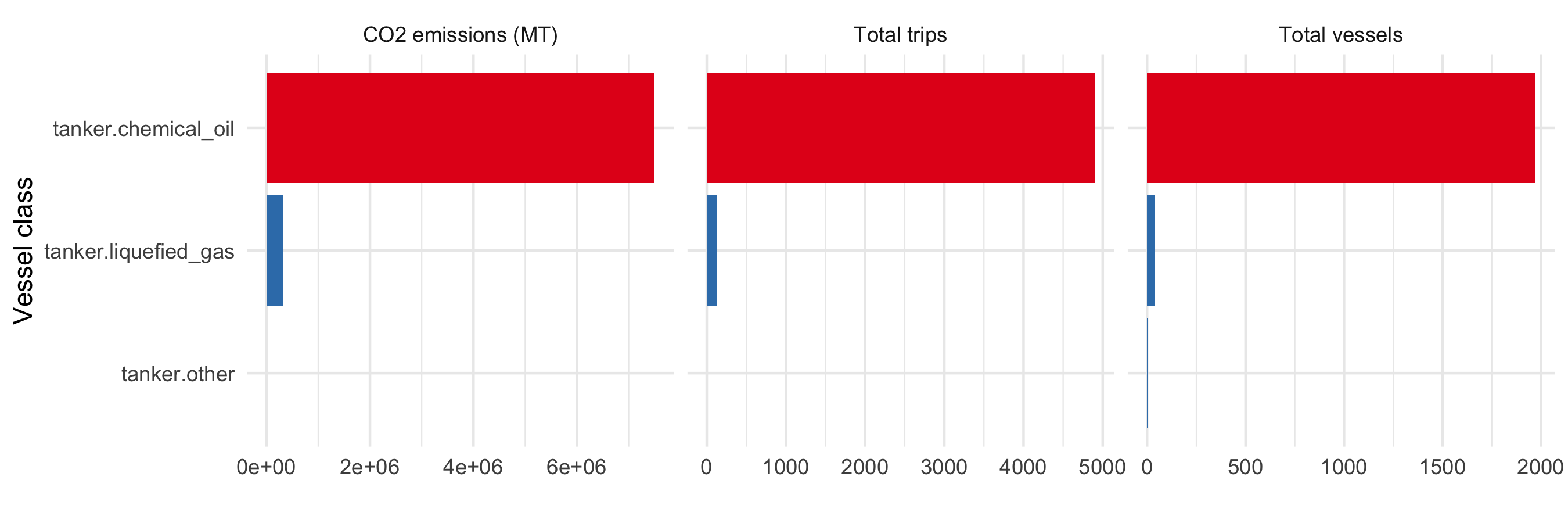
First we look at the total amount of CO2 emissions, number of tanker trips, and number of unique tanker vessels, and for all tanker voyages that end at California ports in our dataset, aggregated by tanker type. The class with by far the most activity is tanker.chemical_oil, which includes crude oil tankers, petroleum product tankers, and chemical tankers. We cannot at this time differentiate further between chemica and oil tankers, but we should eventually have this capability later this year. tanker.liquified_gas are much less common in voyages ending in California.

For the remainder of the analysis after this figure, we will focus on the tanker.chemical_oil class.

tanker_trip_emissions_ending_in_california |>
  dplyr::group_by(vessel_class, class_of_interest) |>
  dplyr::summarise(
    total_trips = dplyr::n_distinct(trip_id),
    total_vessels = dplyr::n_distinct(ssvid),
    emissions_co2_mt = sum(emissions_co2_mt)
  ) |>

  dplyr::arrange(-total_trips) |>
  tidyr::pivot_longer(
    cols = c(total_trips, total_vessels, emissions_co2_mt),
    names_to = "metric",
    values_to = "value"
  ) |>
  dplyr::mutate(
    metric = dplyr::recode(
      metric,
      "emissions_co2_mt" = "CO2 emissions (MT)",
      "total_trips" = "Total trips",
      "total_vessels" = "Total vessels"
    )
  ) |>
  ggplot(aes(
    y = reorder(vessel_class, value),
    x = value,
    fill = class_of_interest
  )) +
  geom_bar(stat = "identity") +
  facet_wrap(~metric, scales = "free_x") +
  theme_minimal() +
  labs(x = "", y = "Vessel class") +
  theme(legend.position = "none") +
  scale_fill_brewer(palette = "Set1", direction = -1)

Figure 1: Summary of CO2 emissions, tanker trips, and unique tanker vessels, by vessel class, for voyages ending at California ports. This aggregates activity from the entire time period of the dataset (January 2015 through February 2026).

country_level_data <- tanker_trip_emissions_ending_in_california |>
  dplyr::filter(vessel_class == vessel_class_of_interest) |>
  dplyr::group_by(from_country, country_of_interest) |>
  dplyr::summarise(
    total_trips = dplyr::n_distinct(trip_id),
    total_vessels = dplyr::n_distinct(ssvid),
    emissions_co2_mt = sum(emissions_co2_mt)
  ) |>
  dplyr::arrange(-total_trips) |>
  dplyr::mutate(rank = dplyr::row_number())

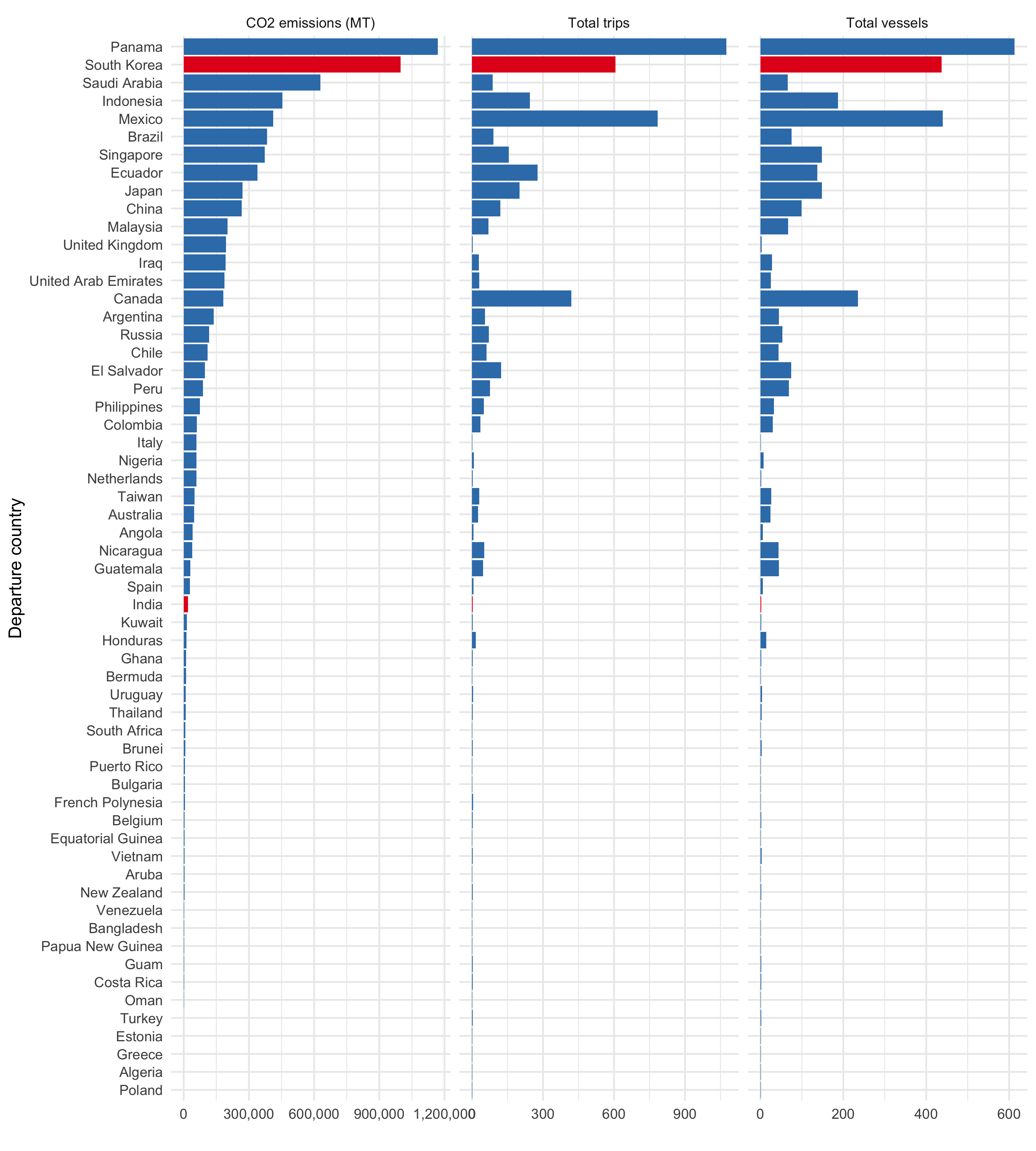
Next we look at the total amount of CO2 emissions, number of tanker trips, and number of unique tanker vessels, and for all chemical and oil tanker voyages that end at California ports in our dataset, aggregated by departure country. In terms of CO2 emissions, our countries of interest, South Korea and India, rank 1 and 1 respectively out of 59 countries with voyages ending in California.

For the remainder of the analysis after this figure, we will focus on voyages departing from our countries of interest, South Korea and India.

country_level_data |>
  tidyr::pivot_longer(
    cols = c(total_trips, total_vessels, emissions_co2_mt),
    names_to = "metric",
    values_to = "value"
  ) |>
  dplyr::mutate(
    metric = dplyr::recode(
      metric,
      "emissions_co2_mt" = "CO2 emissions (MT)",
      "total_trips" = "Total trips",
      "total_vessels" = "Total vessels"
    )
  ) |>
  ggplot(aes(
    y = reorder(from_country, value),
    x = value,
    fill = country_of_interest
  )) +
  geom_bar(stat = "identity") +
  facet_wrap(~metric, scales = "free_x") +
  theme_minimal() +
  labs(x = "", y = "Departure country") +
  theme(legend.position = "none") +
  scale_fill_brewer(palette = "Set1", direction = -1) +
  scale_x_continuous(labels = scales::comma)

Figure 2: Summary of CO2 emissions, tanker trips, and unique tanker vessels, by departure country, for voyages ending at California ports. This aggregates activity from the entire time period of the dataset (January 2015 through February 2026).

# Now, filter to our countries and vessel class of interest for the remainder of the analysis
tanker_trips_of_interest_emissions_ending_in_california <- tanker_trip_emissions_ending_in_california |>
  dplyr::filter(
    vessel_class == vessel_class_of_interest,
    from_country %in% countries_of_interest
  ) |>
  # Make data spatial, using arrival port lat/lon
  sf::st_as_sf(
    coords = c("arrival_lon", "arrival_lat"),
    crs = 4326, # WGS84 coordinate reference system
    remove = FALSE
  ) # Keep original lat/lon columns

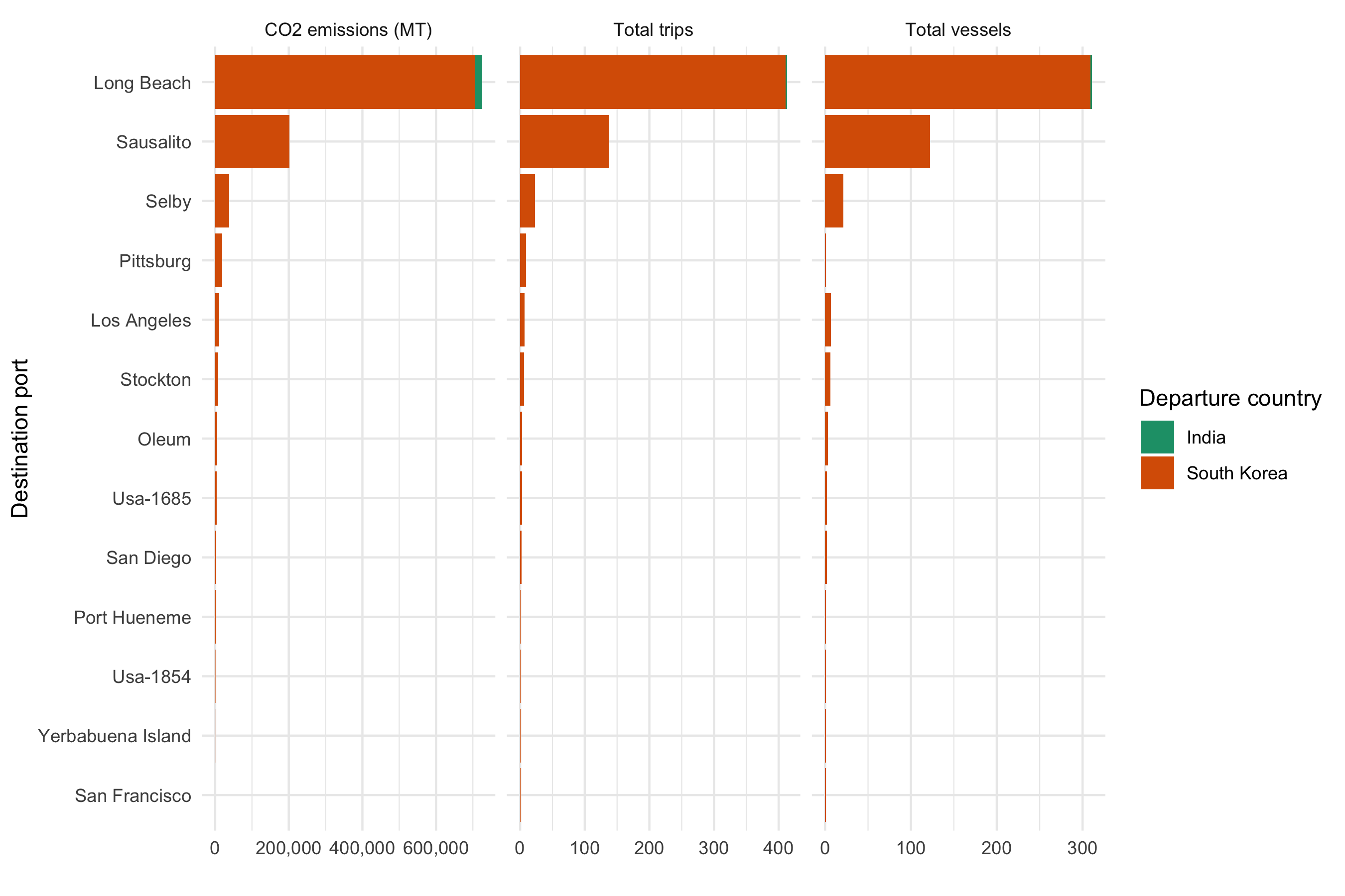
Next we look at the total amount of CO2 emissions, number of tanker trips, and number of unique tanker vessels, for chemical and oil tanker voyages that end at California ports in our dataset, aggregated by departure country and destination port. This allows us to see which California ports are receiving the most tanker traffic and emissions from our countries of interest.

port_level_data <- tanker_trips_of_interest_emissions_ending_in_california |>
  dplyr::mutate(to_port = stringr::str_to_title(to_port)) |>
  dplyr::group_by(to_port, from_country) |>
  dplyr::summarise(
    total_trips = dplyr::n_distinct(trip_id),
    total_vessels = dplyr::n_distinct(ssvid),
    emissions_co2_mt = sum(emissions_co2_mt)
  ) |>
  tidyr::pivot_longer(
    cols = c(total_trips, total_vessels, emissions_co2_mt),
    names_to = "metric",
    values_to = "value"
  ) |>
  dplyr::mutate(
    metric = dplyr::recode(
      metric,
      "emissions_co2_mt" = "CO2 emissions (MT)",
      "total_trips" = "Total trips",
      "total_vessels" = "Total vessels"
    )
  )

port_level_data |>
  ggplot(aes(
    y = reorder(to_port, value),
    x = value,
    fill = from_country
  )) +
  geom_bar(stat = "identity", position = "stack") +
  facet_wrap(~metric, scales = "free_x") +
  theme_minimal() +
  labs(x = "", y = "Destination port", fill = "Departure country") +
  scale_fill_brewer(palette = "Dark2") +
  scale_x_continuous(labels = scales::comma)

Figure 3: Summary of CO2 emissions, tanker trips, and unique tanker vessels, by departure country and destination port, for chemical and oil tanker voyages that end at California ports. This aggregates activity from the entire time period of the dataset (January 2015 through February 2026).

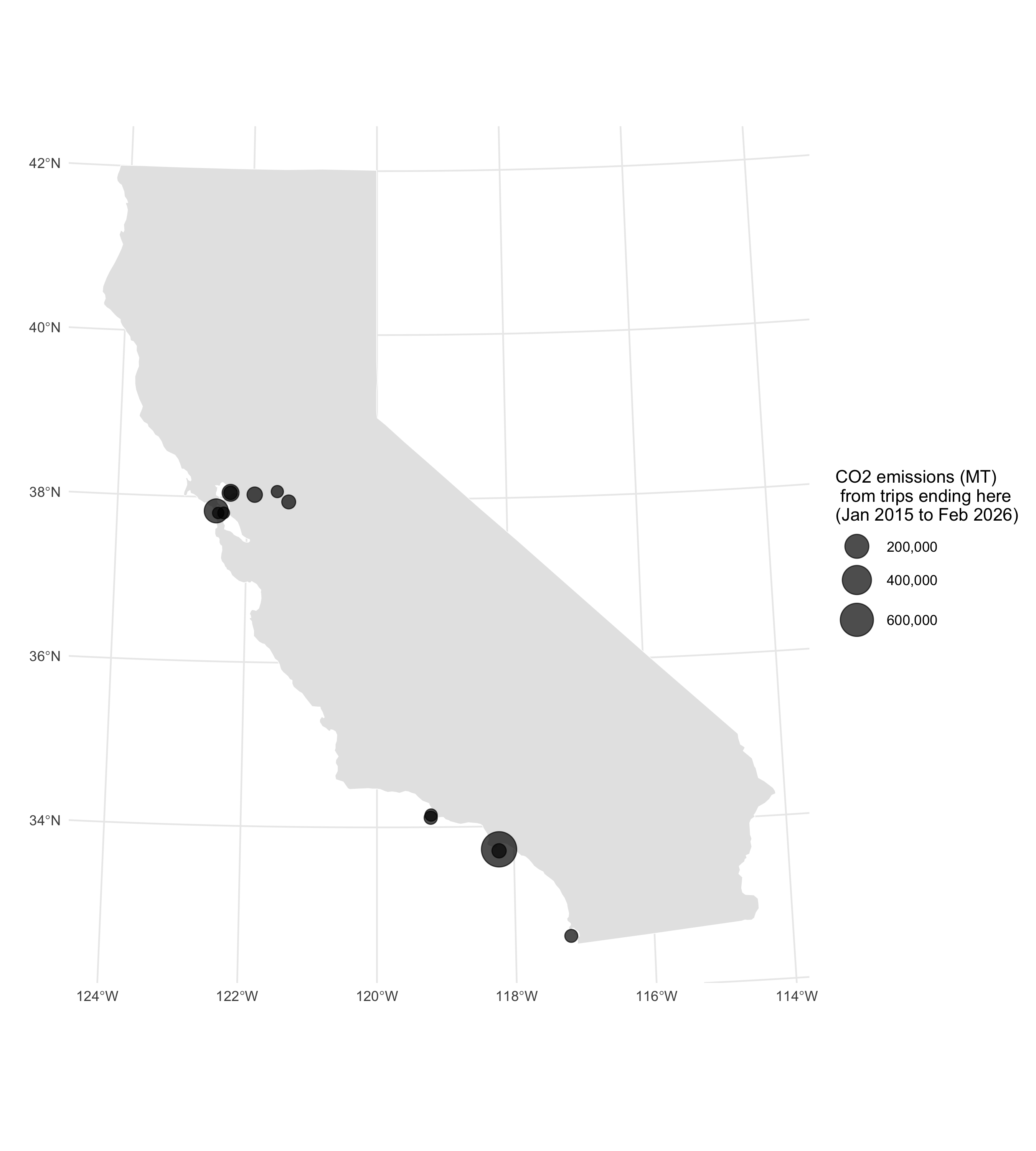
Next we look at a map of the California arrival ports, and how much CO2 emissions are associated with tanker voyages from our countries of interest, South Korea and India, that end at each port. The size of the points corresponds to the amount of CO2 emissions (MT) from voyages departing from each country and arriving at each port.

california_land_mass <- maps::map(
  "state",
  "california",
  plot = FALSE,
  fill = TRUE
) |>
  sf::st_as_sf() |>
  sf::st_transform(crs = 3310)

ggplot() +
  # add California land mass
  geom_sf(
    data = california_land_mass,
    fill = "gray90",
    color = "white"
  ) +
  geom_sf(
    data = tanker_trips_of_interest_emissions_ending_in_california |>
      dplyr::mutate(to_port = stringr::str_to_title(to_port)) |>
      dplyr::group_by(to_port) |>
      dplyr::summarise(
        emissions_co2_mt = sum(emissions_co2_mt),
        geometry = sf::st_union(geometry)
      ) |> # Combine geometries for all trips to the same port
      sf::st_centroid() |> # Get centroid of each port geometry for plotting
      sf::st_transform(crs = 3310), # Transform to California Albers for better visualization,
    aes(size = emissions_co2_mt),
    alpha = 0.7
  ) +
  theme_minimal() +
  labs(
    x = "",
    y = "",
    color = "Departure country",
    size = "CO2 emissions (MT)\n from trips ending here\n(Jan 2015 to Feb 2026)"
  ) +
  scale_color_brewer(palette = "Dark2") +
  scale_size_continuous(
    range = c(3, 10),
    breaks = scales::pretty_breaks(n = 5),
    labels = scales::comma
  ) +
  theme(legend.position = "right")

Figure 4: Map of California arrival ports for chemical and oil tanker voyages from South Korea and India that end at California ports. The point at each point is sized according to how much CO2 emissions occurred on trips from South Korea and India that ended in this port. This aggregates activity from the entire time period of the dataset (January 2015 through February 2026).

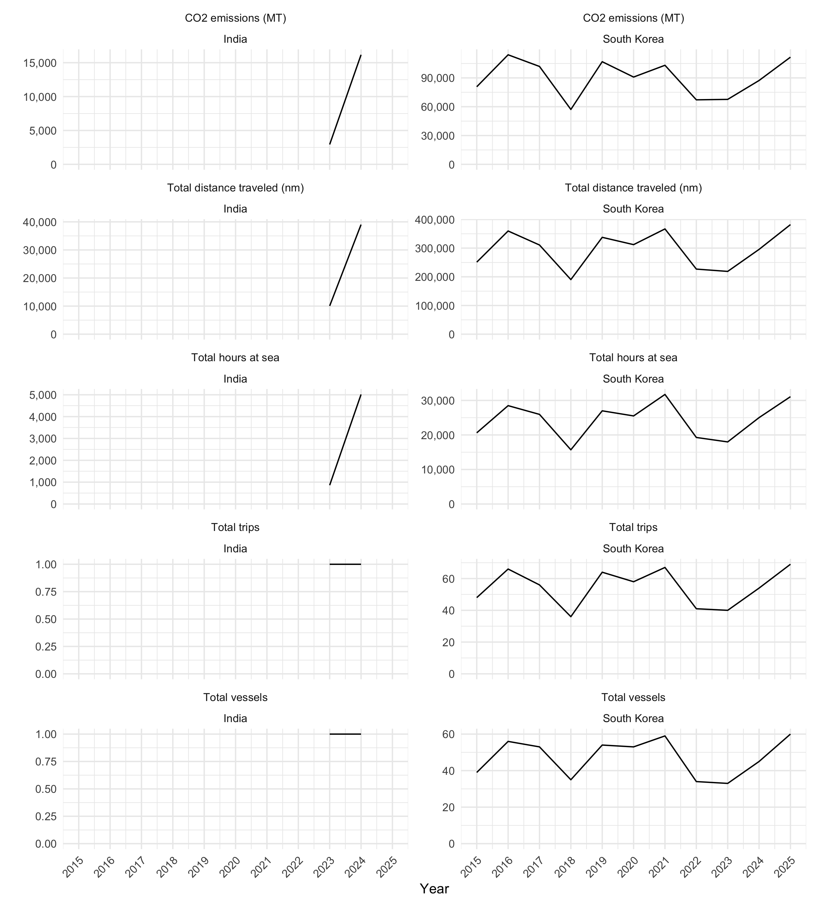
Next we look at a time series plot of number of tanker trips, unique tanker vessels, CO2 emissions, total hours at sea, and total distance traveled (nm), for chemical and oil tanker voyages from South Korea and India that end at California ports. Since 2016 is ongoing, we focus on the 2015-2025 time period. We aggregate by the year during which each voyage arrived in California.

annual_summary_data <- tanker_trips_of_interest_emissions_ending_in_california |>
  sf::st_drop_geometry() |>
  dplyr::filter(vessel_class == vessel_class_of_interest) |>
  dplyr::group_by(
    year = lubridate::year(arrival_date),
    from_country
  ) |>
  dplyr::summarise(
    total_trips = dplyr::n_distinct(trip_id),
    total_vessels = dplyr::n_distinct(ssvid),
    emissions_co2_mt = sum(emissions_co2_mt),
    hours = sum(hours),
    distance_nm = sum(distance_nm)
  ) |>
  dplyr::filter(year < 2026) |>
  tidyr::pivot_longer(
    cols = c(total_trips, total_vessels, emissions_co2_mt, hours, distance_nm),
    names_to = "metric",
    values_to = "value"
  ) |>
  dplyr::mutate(
    metric = dplyr::recode(
      metric,
      "emissions_co2_mt" = "CO2 emissions (MT)",
      "total_trips" = "Total trips",
      "total_vessels" = "Total vessels",
      "hours" = "Total hours at sea",
      "distance_nm" = "Total distance traveled (nm)"
    )
  )
annual_summary_data |>
  ggplot(aes(x = year, y = value)) +
  geom_line() +
  facet_wrap(metric ~ from_country, scales = "free_y", ncol = 2) +
  theme_minimal() +
  labs(x = "Year", y = "", color = "Departure country") +
  scale_color_brewer(palette = "Set1", direction = -1) +
  scale_y_continuous(labels = scales::comma, limits = c(0, NA)) +
  scale_x_continuous(breaks = seq(2015, 2025, by = 1)) +
  theme(axis.text.x = element_text(angle = 45, hjust = 1))

Figure 5: Annual number of tanker trips, unique tanker vessels, CO2 emissions, total hours at sea, and total distance traveled (nm), for chemical and oil tanker voyages from South Korea and India that end at California ports.

Here we summarize this annual data in a table

annual_summary_data |>
  dplyr::mutate(value = round(value) |> prettyNum(big.mark = ",")) |>
  tidyr::pivot_wider(names_from = metric, values_from = value) |>
  dplyr::arrange(from_country, year) |>
  knitr::kable()

Table 1: Annual number of tanker trips, unique tanker vessels, CO2 emissions, total hours at sea, and total distance traveled (nm), for chemical and oil tanker voyages from South Korea and India that end at California ports.

year	from_country	Total trips	Total vessels	CO2 emissions (MT)	Total hours at sea	Total distance traveled (nm)
2023	India	1	1	2,935	861	10,067
2024	India	1	1	16,168	5,015	39,018
2015	South Korea	48	39	80,784	20,617	251,121
2016	South Korea	66	56	114,063	28,485	359,755
2017	South Korea	56	53	101,919	25,955	310,863
2018	South Korea	36	35	57,154	15,697	190,291
2019	South Korea	64	54	106,866	26,986	337,622
2020	South Korea	58	53	90,879	25,506	312,161
2021	South Korea	67	59	103,141	31,729	366,919
2022	South Korea	41	34	67,173	19,272	226,899
2023	South Korea	40	33	67,640	17,982	218,833
2024	South Korea	54	45	87,314	25,020	295,618
2025	South Korea	69	60	111,582	31,080	381,953