4.2 Using BigQuery in R
There is no single best way to access and use GFW data in R. Below are a few techniques that can be used depending on personal preference and project needs. While it is possible to use GFW data without writing SQL using the dbplyr package, this document focuses on workflow to integrate SQL into R.
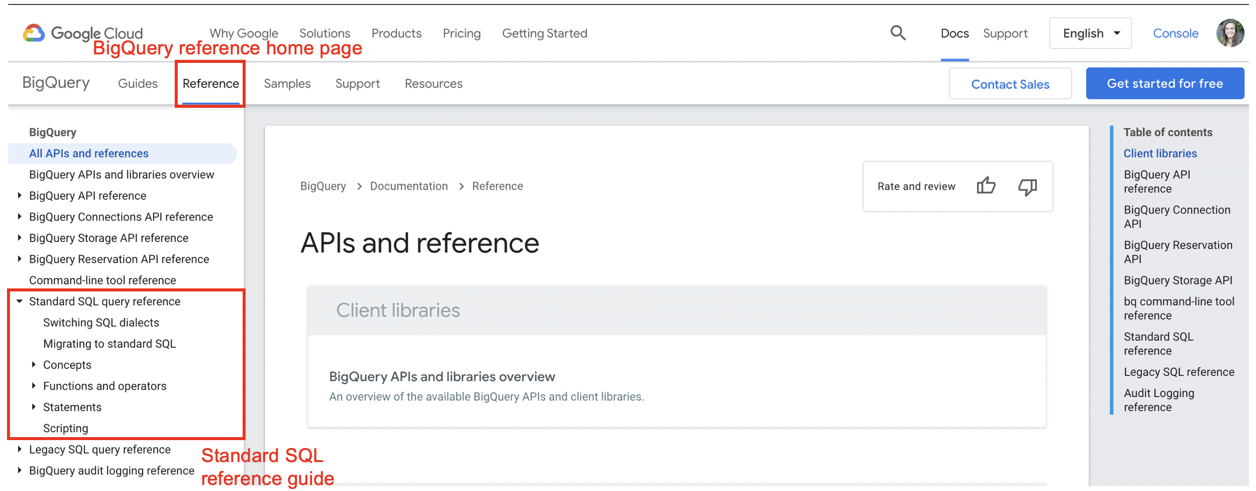
BigQuery can understand both Standard and Legacy SQL. Best practice to use Standard SQL. BigQuery has a very helpful Reference Guide for functions and operators in Standard SQL. In particular, the ‘Functions and Operators’ section, found under the ‘Standard SQL query reference’ heading, contains helpful documentation on a range of functions categorized by type.
4.2.2 Accessing Data
When writing SQL, data can be accessed using three pieces of information: the project, the dataset, and the table. This should follow the syntax project.dataset.table. Specifying the project first is important. SQL will only be able to find datasets and tables within the billing project (e.g. emlab-gcp) if no project is specified. For example when emlab-gcp is set as the billing project, trying to access the eez_info table using gfw_research.eez_info produces an error that the table does not exist. Adding the project first, world-fishing-827.gfw_research.eez_info fixes the query.
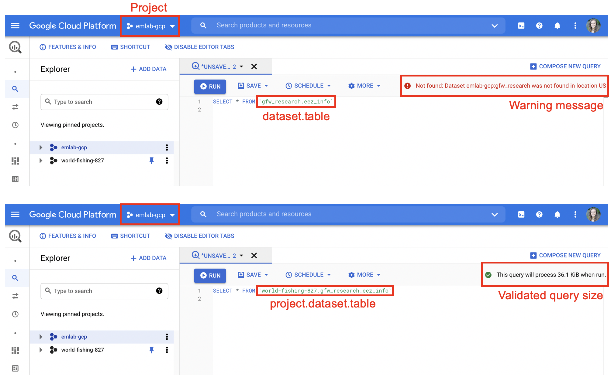
Best practice is to always specify the project since this reduces potential errors if others replicate your code using a different billing project.
4.2.3 Writing and Executing Queries
There are two main methods for executing SQL in R. One is to write the SQL query as a string and then execute it using the bigrquery or DBI packages. The second is to use an SQL chunk within your markdown or notebook. The following libraries are useful for accessing GFW data: DBI, bigrquery, glue.
Writing Queries as Strings
Queries can be written as strings in R. Best practice is to avoid looped or nested queries and instead use subqueries. Subqueries can be written using ‘WITH’ statements.
#############################################################
# Example Query: Find which EEZs vessels fished in
# Description:
# This query uses the vessel info table to identify all vessels
# that fished in China each year and how much they fished.
#############################################################

sql_vessels_in_china <- "#StandardSQL

WITH

  ###############################
  # Get EEZ ID and info

  eez_names AS (
  SELECT
    CAST(eez_id AS STRING) AS eez,
    reporting_name,
    sovereign1_iso3 AS eez_iso3
  FROM
    `world-fishing-827.gfw_research.eez_info`),

  ###############################
  # Get EEZ fishing summary from activity.eez array

  eez_fishing AS (
  SELECT
    ssvid,
    year,
    best.best_flag,
    best.best_vessel_class,
    value AS eez,
    fishing_hours
  FROM
    `world-fishing-827.gfw_research.vi_ssvid_byyear_v20201209`
  CROSS JOIN
    UNNEST(activity.eez)
  WHERE on_fishing_list_best),

  ###############################
  # Join country name to EEZ id

  eez_fishing_labeled AS (
  SELECT
    *
  FROM
    eez_fishing
  JOIN
    eez_names
  USING
    (eez)),

  ###############################
  # Filter to fishing in China using ISO3

  chn_fishing AS (
  SELECT
    *
  FROM
    eez_fishing_labeled
  WHERE
    eez_iso3 = 'CHN'
    AND fishing_hours > 0)

  ###############################

  SELECT * FROM chn_fishing"
The query can be run using the bigrquery package or the DBI package. When using bigrquery, the bq_project_query() function enables you to run the query and only requires the billing code and the query string. This function will not download the results of your query. To run the query and download results locally you can combine the bq_project_query() and bq_table_download() functions. More information is available in the package documentation.
# Run query only - stores results to a temporary table in BigQuery
bq_project_query("emlab-gcp", sql_vessels_in_china)

# Run query and download results
vessels_in_china <- bq_project_query("emlab-gcp", sql_vessels_in_china) %>%
  bq_table_download(max_results = Inf)
A second option is to connect to BigQuery using the DBI package. When using DBI you first setup the connection using dbConnect() and then you can run your query using dbGetQuery(). The connection requires the driver (BigQuery), project name, and billing code. More information about DBI is available in the package documentation.
# Set up connection
bq_connection <- dbConnect(
    bigquery(),
    project = "world-fishing-827",
    billing = "emlab-gcp"
)

# Run query
vessels_in_china <- dbGetQuery(bq_connection, sql_vessels_in_china)
Writing Queries Using glue
Using glue::glue_sql() allows for substitution of R variables into the query. Substitute R variables into the query using {variable}. Be aware of proper syntax: substituting characters requires using back ticks but numbers or integers don’t. This might be useful if, for example, you want to run the same query for different years. Using glue_sql() requires adding the connection using the .con arguument after the query string. The connection is established in the same way as above, using dbConnect(). The query can then be run using either DBI or bigrquery as shown above.
#############################################################
# Example Query: Find which EEZs vessels fished in annually
# Description:
# This query uses the vessel info table to identify all vessels
# that fished in China in 2019 and how much they fished.
#############################################################


# Define variables
country <- 'CHN'
year    <- 2019

# Write query

sql_vessels_in_china <- glue_sql("#StandardSQL

WITH

  ###############################
  # Get EEZ ID and info

  eez_names AS (
  SELECT
    CAST(eez_id AS STRING) AS eez,
    reporting_name,
    sovereign1_iso3 AS eez_iso3
  FROM
    `world-fishing-827.gfw_research.eez_info`),

  ###############################
  # Get EEZ fishing summary from activity.eez array

  eez_fishing AS (
  SELECT
    ssvid,
    year,
    best.best_flag,
    best.best_vessel_class,
    value AS eez,
    fishing_hours
  FROM
    `world-fishing-827.gfw_research.vi_ssvid_byyear_v20201209`
  CROSS JOIN
    UNNEST(activity.eez)
  WHERE on_fishing_list_best
  AND year = {year}),

  ###############################
  # Join country name to EEZ id

  eez_fishing_labeled AS (
  SELECT
    *
  FROM
    eez_fishing
  JOIN
    eez_names
  USING
    (eez)),

  ###############################
  # Filter to fishing in China using ISO3

  chn_fishing AS (
  SELECT
    *
  FROM
    eez_fishing_labeled
  WHERE
    eez_iso3 = {`country`}
    AND fishing_hours > 0)

  ###############################

  SELECT * FROM chn_fishing", .con = bq_connection)

# Run query
vessels_in_china_2019 <- bq_project_query("emlab-gcp", sql_vessels_in_china) %>%
  bq_table_download(max_results = Inf)
Using SQL Chunks
Both R markdown and R notebooks allow for integration of prose and different programming languages, such as python or SQL, within one document. Selecting “Insert → SQL” will add a code chunk to the document and enable you to write in SQL directly instead of saving the query as a string. In SQL chunks instead of using # to annotate, comments should be enclosed by /* */ (i.e. /* Comment */).
When using SQL code chunks, it is important to specify the database connection and the output variable within the top of the code chunk. The database connection is established in the same way as shown above with DBI::dbConnect(). After running the code chunk, the results should appear in the enviroment using the name of the output variable.
WITH

  /* Get EEZ id and info */

  eez_names AS (
  SELECT
    CAST(eez_id AS STRING) AS eez,
    reporting_name,
    sovereign1_iso3 AS eez_iso3
  FROM
    `world-fishing-827.gfw_research.eez_info`),

  /* Get EEZ fishing summary from activity.eez array */

  eez_fishing AS (
  SELECT
    ssvid,
    year,
    best.best_flag,
    best.best_vessel_class,
    value AS eez,
    fishing_hours
  FROM
    `world-fishing-827.gfw_research.vi_ssvid_byyear_v20201209`
  CROSS JOIN
    UNNEST(activity.eez)
  WHERE on_fishing_list_best),

  /* Join country name to EEZ id */

  eez_fishing_labeled AS (
  SELECT
    *
  FROM
    eez_fishing
  JOIN
    eez_names
  USING
    (eez)),

  /* Filter to fishing in China using ISO3 */

  chn_fishing AS (
  SELECT
    *
  FROM
    eez_fishing_labeled
  WHERE
    eez_iso3 = 'CHN'
    AND fishing_hours > 0)

  /* Select the final query */

  SELECT * FROM chn_fishing
4.2.4 Subsetting Data
Some queries may be expensive to run and output large amounts of data. To check results from queries or to make sure they work correctly, it may be necessary to subset the data. Tables that are partitioned are divided up into smaller segments and can be easily subsetted to reduce query size and cost. A common technique for testing queries is to restrict the date range to a single day. This can be accomplished using WHERE plus a date filter (like _PARTITIONTIME) although the specific notation will depend on if the data are represented as a date or a timestamp.
Another option to test queries is to use the emlab-gcp.emlab_test dataset. This dataset holds a smaller version of the
gfw_research.pipe_vYYYYMMDD_fishing table containing only data from 2020. This table is meant to allow for testing and checking query results before a full query is run using the pipe_vYYYYMMDD_fishing table. The table pipe_v20201001_fishing_subset2020 is still 485.5 GB so it’s recommended to further subset the table when testing out queries.
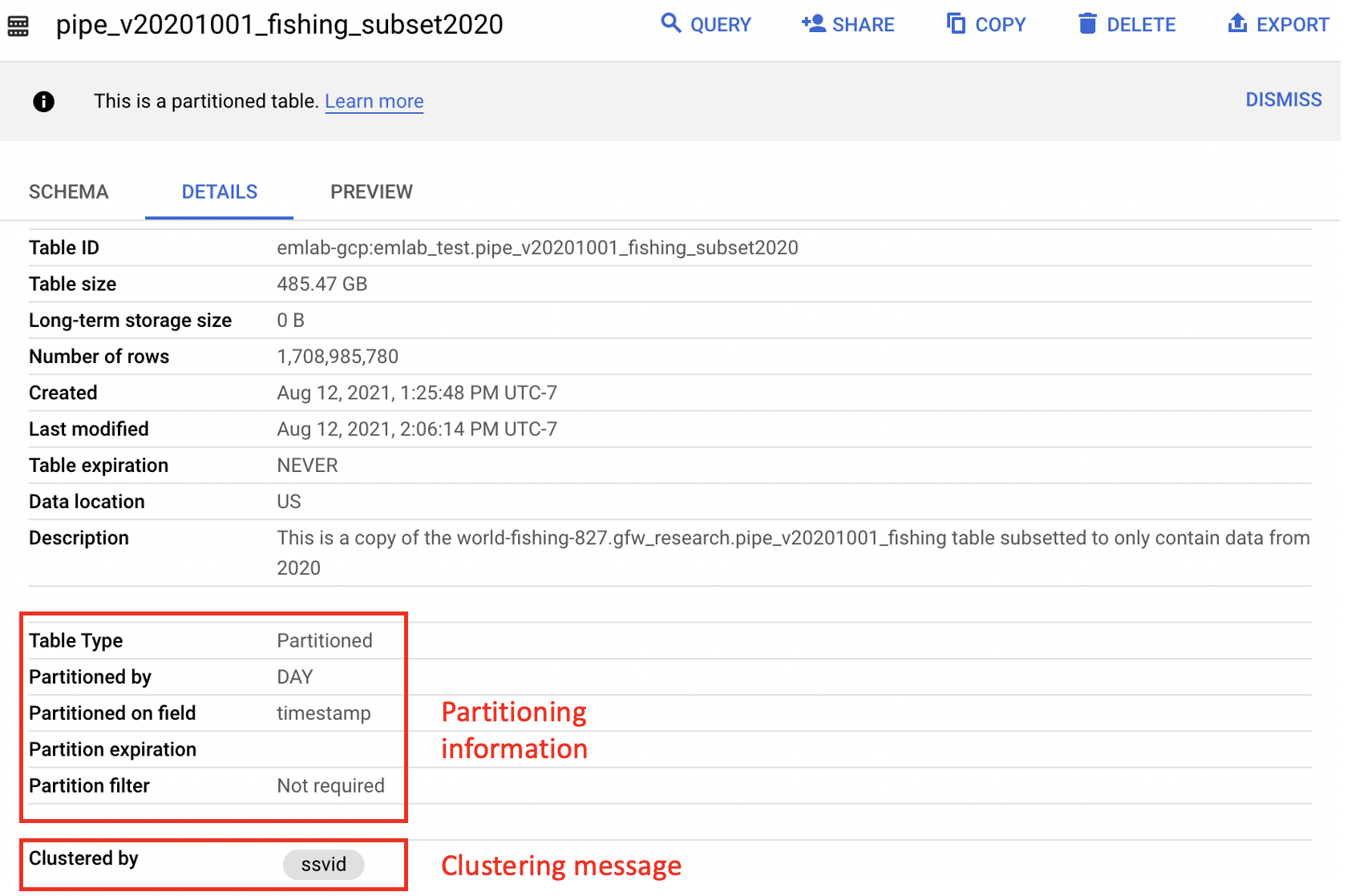
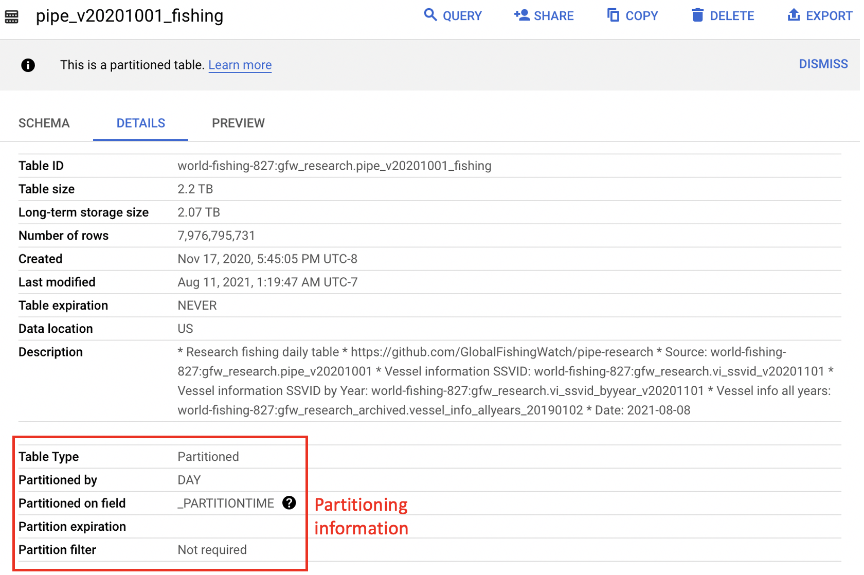
Generally, partitioned tables are noted in BigQuery with a message under the ‘Details’ tab and more information about how the table is partitioned is available in the Table Info. In particular, the partitioned on field lets the user know what the partitioning field is which can help determine the proper syntax. The figure below illustrates the difference in partitioning fields between the source pipe_v20201001_fishing table and the pipe_v20201001_fishing_subset2020 table. The Table Info for the world-fishing-827.gfw_research.pipe_v20201001_fishing table indicates it is partioned on _PARTITIONTIME, which makes WHERE _PARTITIONTIME = 'date' the proper syntax for querying a single day of data from this table as illustrated in the example below. The emlab-gcp.emlab_test.pipe_v20201001_fishing_subset2020 Table Info shows the partitioning field is timestamp which makes WHERE timestamp = 'date' the correct way to filter for a single day of data. An example of querying fishing effort using this test table is provided in Section 4.3. Partitioning will have the lagest impact on query size but there are other ways to reduce the size and cost of your queries including selecting only columns you need and filtering based on clustered columns (such as ssvid in the pipe_vYYYYMMDD_fishing table). The clustered columns are also noted in the Table Info below the partitioning section and more information on how clustering reduces query size and cost can be found in the BigQuery documentation. GFW tables that are partioned are also noted in the table descriptions in Section 3 and more information on partioned tables can be found in the BigQuery documentation.
#############################################################
# Example Query: Fishing hours for January 1, 2019
# Description:
# This query uses the fishing table to calculate fishing
# hours January 1, 2019.
#############################################################

sql_fishing_hours <- "#StandardSQL

WITH

  ###############################
  # Find good segments

  good_segments AS (
  SELECT
    seg_id
  FROM
    world-fishing-827.gfw_research.pipe_v20201001_segs
  WHERE
    good_seg
    AND positions > 10
    AND NOT overlapping_and_short),

  #######################
  # Active non-noise fishing vessels

  fishing_vessels AS (
  SELECT
    *
  FROM
    world-fishing-827.gfw_research.fishing_vessels_ssvid_v20201209
  WHERE
    year = 2019),

  ###############################
  # Find fishing hours

  fishing_hours AS (
  SELECT
    ssvid,
    timestamp,
    lat,
    lon,
    hours,
    IF(nnet_score > 1, hours, 0) AS fishing_hours
  FROM
    world-fishing-827.gfw_research.pipe_v20201001_fishing
  WHERE
    _PARTITIONTIME = '2019-01-01'
  AND seg_id IN (
    SELECT
      seg_id
    FROM
      good_segments)
  AND ssvid IN (
    SELECT
      ssvid
    FROM
      fishing_vessels))

  ###############################

  SELECT * FROM fishing_hours"
4.2.5 Saving / Downloading BigQuery Tables
In some cases you might want to save your query results directly to BigQuery. For example, it may be easier to store large tables in BigQuery than trying to work with large amounts of data in R. A large table can then be further queried and subsetted before working with the data in R. Additionally, it may be useful to store tables in BigQuery if you plan to join them with other data stored in BigQuery. For instance, a table of spatial boundaries may be useful to store on BigQuery for spatially filtering data from other BigQuery tables to a specific region of interest. Tables can be saved to BigQuery using either bigrquery::bq_project_query() or DBI::dbWriteTable(). Using the bq_project_query() function allows you to execute the query and save the results as a new table in BigQuery in a single step by adding the destination_table argument. When using DBI you need to execute the query first and then write the results to the database.
Datasets and tables should only be created in the emlab-gcp project. Datasets need to be created before tables can be saved there and can be created in the BigQuery console or in R using bq_dataset_create(). In the BigQuery console datasets can be created by navigating to the emlab-gcp project and selecting the ‘Create Dataset’ button. The default settings for creating the dataset are fine to keep, only the dataset name needs to be added. Once the dataset is created, refreshing the window should show the new dataset on the left hand side nested under the emlab-gcp project.
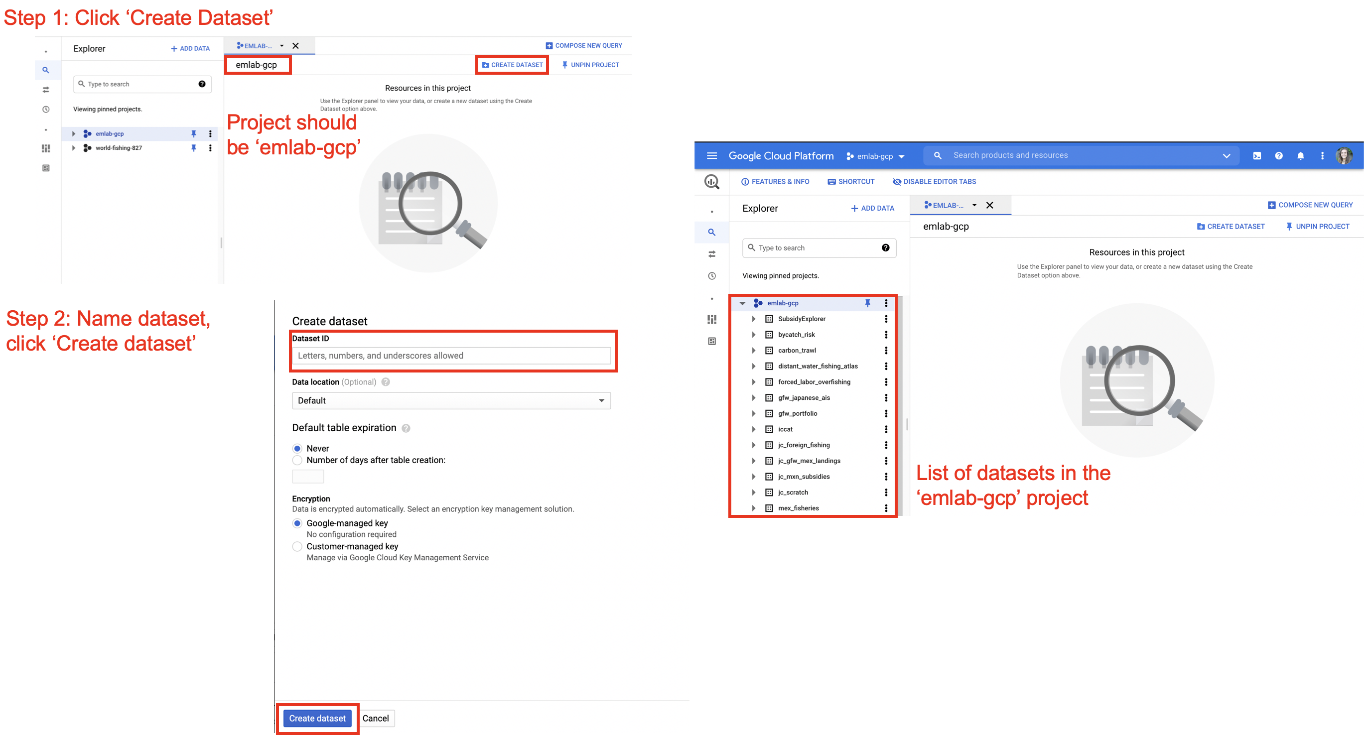
Best practices for naming datasets is to use the official project name, the same one used for the GitHub respository, Google Drive, and other project materials. For tables, names should be descriptive and meaningful. It is advised to follow them emLab SOP guidance in Section 3.1 for file naming, specifically using only lower case letters, using ’_’ to separate words, and avoiding ‘-’, ‘.’ and other special characters. After tables are created it’s recommended to go to the BigQuery console and update the description and schema of the table. Providing a link in the description to the markdown file with the query used to generate the table is helpful for reproducibility in future.
bq_project_query("emlab-gcp",
                 sql_fishing_hours,
                 destination_table = bq_table(project = "emlab-gcp",
                                              table = "fishing_hours_20190101",
                                              dataset = "project_name"),
                 use_legacy_sql = FALSE, allowLargeResults = TRUE))
These tables now live in BigQuery. If you return to the BigQuery console and refresh it, you should see the table nested under emlab-gcp and the dataset name.
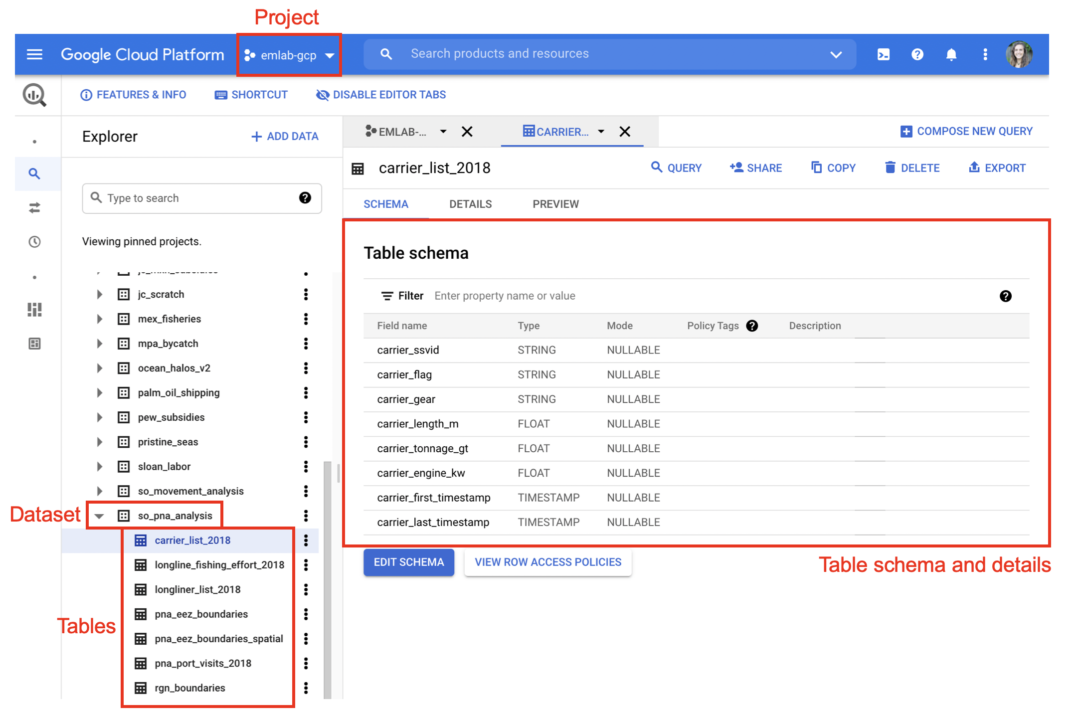
These tables can now be called directly in future queries and can be downloaded in R at any time using either bigrquery::bq_table_download() or DBI::dbReadTable().
# Download table using bigrquery
fishing_hours <- bq_table_download("emlab-gcp.project_name.fishing_hours_20190101",
                                   max_results = Inf)

# Download table using DBI
# Establish a connection to the emlab-gcp project where your table is saved
bq_connection <- dbConnect(
    bigquery(),
    project = "emlab-gcp",
    billing = "emlab-gcp"
)

fishing_hours_dbi <- dbReadTable(bq_connection,
                                 "emlab-gcp.project_name.fishing_hours_20190101")
It is important to remember to save any data at the end of the R session to avoid having to re-run queries every time you open the project.