1  Spatial extend

The spatial domain of DISPLACE is represented by a network of nodes on which simulated vessels navigate and fish. The extent of this domain must be defined based on historical fishing effort and the harbors from which vessels operate. This section provides context on the inputs required to define the study’s spatial domain.

1.1 Graph of nodes

The DISPLACE project provides tutorials on using DISPLACE. Among them is a guide to setting up a new graph of nodes that explains step by step how to use the DISPLACE GUI to create the node graph, an input required by the R routines and the model.

To do so, at least two .shp files are required: one defining the area extent for simulating vessel behavior, and an inverted shape to prevent the generation of nodes outside the area of interest. Example files are provided in this repository under raw_inputs/GRAPH/shp as graph_area.shp and exclusion_area.shp. Using these, you can generate the graph of nodes, which is already available for this example application in raw_inputs/GRAPH as graph0.dat and its associated files.

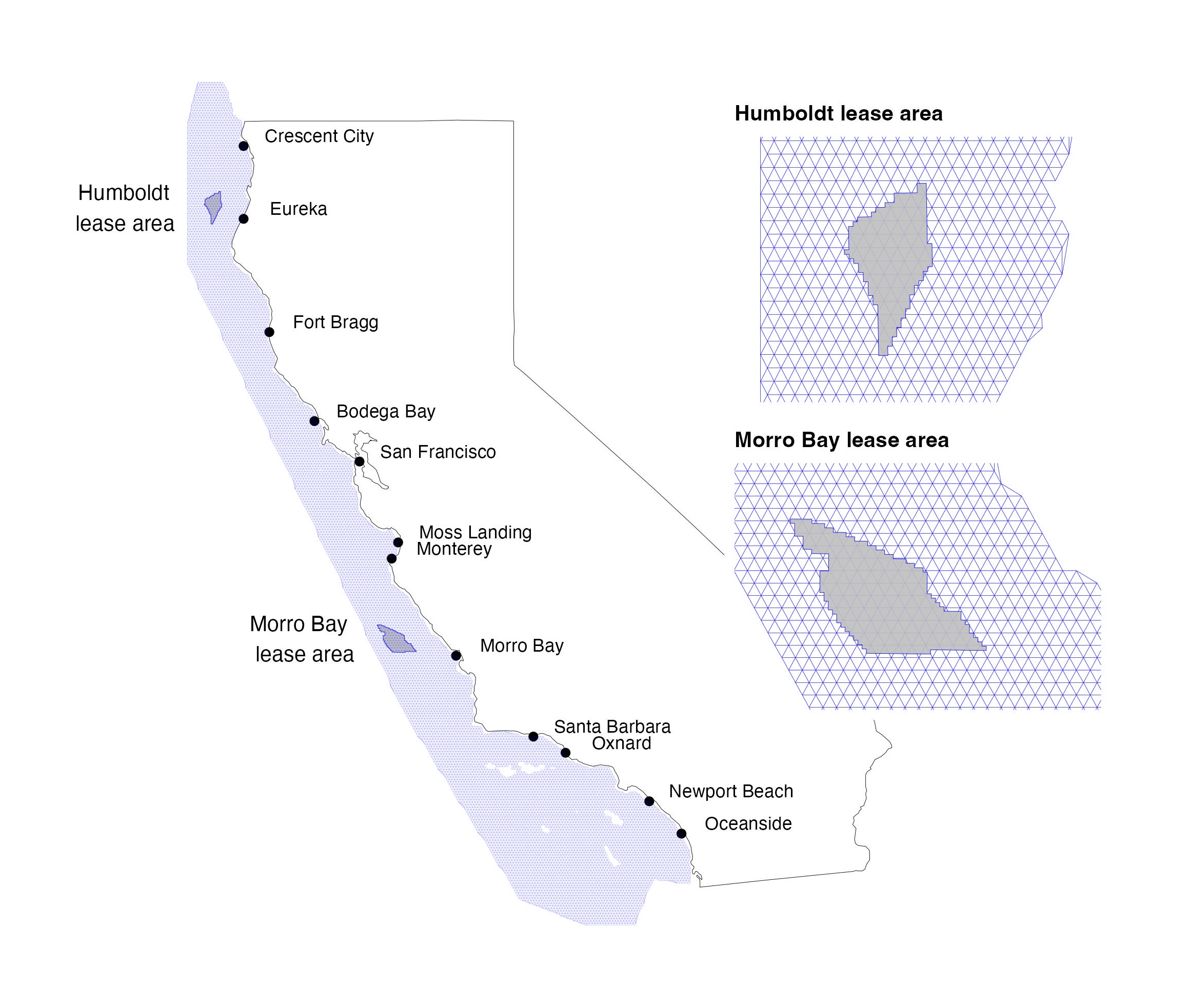
For this study, we focus on the waters off the coast of California using a spatial domain that spans latitudinally from roughly the US/Mexico EEZ border to Cape Blanco (32.0° to 42.6°) and longitudinally from -125.1° to -117.3°. Nodes are 4 km apart (Figure 1.1).

Figure 1.1: DISPLACE study area. The spatial extent for this study is determined by the spatial distribution of DTS vessel fishing effort, informed by the merged VMS-fish ticket dataset. This results in a latitudinal extent of 32.0° to 42.6°, and longitudinal extent of -125.1° to -117.3°. Nodes are 4 km apart, and the twelve ports depicted are those included in the simulations. OSW areas are shaded in grey.

1.2 Harbors

As detailed in the graph of nodes tutorial the generated nodes of the stidy area (graph0.dat) need to be associated to the harbors from where the vessels operate in the simulation. Such, vessels need to be specified in the file GRAPH/harbours.dat, with the port name with no blank spaces, a port id and the latitude and lon coordinates as shown in Table 1.1.

Table 1.1: Details of the harbour.dat file contents for this case study.

port_name	lon	lat	idx_port
Crescent_City	-124.2	41.7	1
Eureka	-124.2	40.8	2
Fort_Bragg	-123.8	39.4	3
Bodega_Bay	-123.1	38.3	5
San_Francisco	-122.4	37.8	4
Moss_Landing	-121.8	36.8	7
Monterey	-121.9	36.6	6
Morro_Bay	-120.9	35.4	8
Santa_Barbara	-119.7	34.4	10
Oxnard	-119.2	34.2	9
Newport_Beach	-117.9	33.6	11
Oceanside	-117.4	33.2	12

The final updated graph, with nodes connected to the ports of interest, has already been generated and is available at GRAPH/graph1.dat along with its associated files. This is the graph that will be used to run DISPLACE. Additionally, GRAPH/graph2.dat contains the updated graph that defines the lease areas closure scenario.