1  Populations data

1.1 Populations

This section includes a description of the raw input datasets and the parameters considered to run the R routines for the target species population characteristics. These files should be stored and loaded from DISPLACE_raw_inputs/{project-name}/POPULATIONS.

Commercial species included in this study:

• Sablefish (Anoplopoma fimbria) (FAO code SAB): Status along the U.S. West Coast in 2023.
• Dover Sole (Microstomus pacificus) (FAO code MIP): Stock assessment along the U.S. West Coast in 2021.
• Longspine Thornyhead (Sebastolobus altivelis) (FAO code SJZ): Biological data from stock assessments in California, Oregon, and Washington in 2013.
• Shortspine Thornyhead (Sebastolobus alascanus) (FAO code SJU): Status along the U.S. West Coast in 2023.

We are focusing on these species because, aside from albacore—which we can’t model due to the fishery’s range—they are the most common in the lease areas. While swordfish is also common, its fishery is about to close, so we did not include it. These species also represent the highest landings by weight and value (though sablefish prices have recently dropped). Although crab and squid have the highest overall landings, they are primarily caught nearshore and are therefore not impacted by the leases. The fisheries of this species is also known ans DTS (Deepwater Trawl complex Species).

1.2 Stock biological traits

This section describes the contents of the file Stock_biological_traits.csv. Most of the data is extracted from the stock assessments approved by the Pacific Fishery Management Council during the September 2023 Council Meeting.

Besides specific parameter values for each species, detailed in the subsequent sections, the following variables are also included in Stock_biological_traits.csv:

• UseIt: values Yes/No, indicating whether it is included in the analysis or not.
• stock: code of the population. For our study case this corresponds to the FAO code.
• species: Species scientific name.
• Source_Biology and Source_Stock: references from where the values are taken.

Stock_biological_traits.csv also contains details on the input size bins in DISPLACE, as defined in Stock_abundances_at_szgroup.csv.Using the maximum length values across all DTS species, we set a sz_bin_cm of 6 (in cm) based on the unit_sizebin, where a value of 1 is used. For more details, refer to the section on abundance by size.

1.2.1 Sablefish

(Anoplopoma fimbria) (FAO code SAB)

---

Note: For cases with sexual dimorphism, the average value across both females and males is used.

1.2.1.1 Somatic growth

• Linf: Asymptotic length. Sablefish stock assessments assumes Schnute growth rather than von Bertalanffy growth. Since DISPLACE does not incorporate Schnute, we will derive Bertalanffy parameters from those in Schnute.

  The von Bertalanffy growth function is given by the folowwing expression:

\[ L(t)=L_∞(1−e^{−K(t−t_0)}) \]

The four-parameter growth function from Schnute can be defined as:

\[ L(t) = L_1 + \left( L_2 - L_1 \right) \frac{1 - e^{-K(t - t_1)}}{1 - e^{-K(t_2 - t_1)}} \]

Table 1.1: Schnute and von Bertalanffy growth parameters for Sablefish.

Parameter	Value
Length-at-age min (female)	25.262
Length-at-age max (female)	61.130
von Bertalanffy K (female)	0.367
Length-at-age min (male)	26.621
Length-at-age max (male)	56.111
von Bertalanffy K (male)	0.381

We can get \(L_2\) from Length-at-age max (female) is 61.130 and (male) 56.111, and \(L_1\) from Length-at-age max (female) is 25.262 and (male) 26.621 in page 27, table 2 (Johnson, Wetzel, and Tolimieri (2023)). Further, \(K\) corresponds to 0.367 \(yr^{-1}\) for females and 0.381 \(yr^{-1}\) for males from page 10 and from von Bertalanffy K variables in page 27, table 2 (Johnson, Wetzel, and Tolimieri (2023)) (Table 1.1). Regarding \(t_1\) and \(t_2\), these can be found on the benchmark assessment M. A. Haltuch et al. (2019), section 3.3, page 54, on general model specifications, corresponding to 0.5 and 30 years respectively.

If we derive LInf from Schnute we get:

\[ L_{\infty} = \frac{L_2 - L_1 \cdot e^{-K(t_2 - t_1)}}{1 - e^{-K(t_2 - t_1)}} \]

Based on the parameters available in the assessment, we will calculate Linf independently for males and females. The average value across both will be inputted into DISPLACE and corresponds to 58.6210501.

Alternatively, if the values from the stock assessment could not be derived, we could have considered using the value of 63.67 cm from Table 6 in M. A. Head, Keller, and Bradburn (2014) publication. However, we are including these here merely as a reference.

• CV_Linf: We only have Schnute parameters available. In this case, we will use the average of the Growth CV old values, as they are the closest to Linf and can serve as a proxy. These correspond to Growth CV old (female) (0.103) and (male) (0.078) in page 27, table 2 (Johnson, Wetzel, and Tolimieri (2023)). Mean value used 0.0905.

• K: Von Bertalanffy \(K\). 0.367 \(yr^{-1}\) for females and 0.381 \(yr^{-1}\) for males from page 10 and from von Bertalanffy K variables in page 27, table 2 (Johnson, Wetzel, and Tolimieri (2023)). Mean value used 0.374 \(yr^{-1}\).

• t0: Theoretical age of the von Bertalanffy growth function (VBGF) at which fish would have a size of zero. Again, we need to consider that the stock assessment express growth using Schnute parameters. Thus we’ll need to derive \(t_0\) from:

\[ t_0 = t_1 + \frac{1}{K} \ln \left( \frac{L_2 - L_1}{L_2 - L_1 \cdot e^{-K(t_2 - t_1)}} \right) \]

This yields a t0 of -1.1883843, which we will use. For reference, Table 7 from M. A. Head, Keller, and Bradburn (2014) provides an overall estimate of -1.28 years. TO DISCUSS

• CV_recru: Coefficient of variation in recruitment. Table 2, on page 27 from the stock assessment, includes all model parameters. Among others, it defines recruitment variability (\(\sigma R\)), which corresponds to the standard deviation of the log-scale recruitment deviations (Johnson, Wetzel, and Tolimieri (2023)). Then the coefficient of variation (CV) of recruitment can be estimated from this parameter as follows:

\[ CV = \sqrt{ \exp(\sigma R^2) - 1 } \]

Thus, for \(\sigma R = 1.4\), the CV will be 2.4696816.

1.2.1.2 Length-weight relationship

Length-weight relationship expression: \(W = aL^b\)

• a: Weight-length coefficient. Female 3.315e-06 and male 3.371e-06 from table 11 (M. Haltuch et al. (2019)). Mean value used 3.343^{-6}.

• b: Weight-length exponent. Female 3.27264 and male 3.27008 from table 11 (M. Haltuch et al. (2019)). Mean value used 3.27136.

1.2.1.3 Maturity

• L50: Length 50% mature. Overall value of 54.64 cm (used in Marlin) from all geographic areas and depths combined from Table 3 (M. A. Head, Keller, and Bradburn (2014)). Alternative value of 55.190 from table 11 (M. Haltuch et al. (2019)). Both values correspond to female lengths. We will use the average from both assessments.

  To determine the male’s L50, we can use the proportion of L50 to Linf observed in females. Given that the female Linf is 61.130 cm and the female L50 is 54.915 cm (from the average of the available values), we first calculate the proportion of L50to Linf for females (0.8983314). We then apply this same proportion to the male Linf (56.111 cm) to find the male L50 (50.4062746cm). We will use the mean value between female and the calcualted male lengths 52.6606373 cm. (This value is also given to the DISPLACE parameter mat).

• mat_cat: This corresponds to the maturity size DISPLACE category at the L50. Given 0:13 bins and a sz_bin_cm of 6, as defined earlier, the corresponding bin index for an L50 of 52.6606373 cm is 9.

  NOTE: Bastardie described it with the following example: if there are 5 cm bins (0, 1, 2, 3, 4, 5) and the L50 maturity size is 14 cm, then the mat_cat should be 3. However, this raises the question: does mat_cat = 3 correspond to the third bin (index 2 in zero-based indexing)? Or should it instead be recoded to 2 to consider initial value of zero?

• r_age: Age of recruitment. (Not used in DISPLACE, but included in the input files as a reference). As a reference here we will use A50, having a value of 6.86 from table 5 (M. A. Head, Keller, and Bradburn (2014)) and a value of 5 from Guzmán et al. (2017), yielding an average value of 5.93, corresponding to the one used in Marlin. We should note that Guzmán et al. (2017) value is not based on their own data but on two outdated paper estimates (Fujiwara and Hankin (1988) and Parks and Shaw (1987)). Alternatively we could also use Rodgveller, Stark, and Echave (2016) values from table 2, although these are specific from Alaska populations. Since DISPLACE does not require this parameter, we will exclusively reference that from M. A. Head, Keller, and Bradburn (2014).

  Note: Despite not being used for DISPLACE parametrization, the parameter is read and it is used within GeneratePopulationsFeatures.R. High values trigger Error in As[r_age + 1, ] : subscript out of bounds associated to line 552 of the R routine. Thus we will specify NA and no A50 value as a reference. Need to confirm with Bastardie whether this is actually affecting the parametrization.

• ssb_assessment: Total weight of the sexually mature (i.e., capable of reproduction) part of a fish population. Spawning Stock Biomass in mT from page 38, table 4 (Johnson, Wetzel, and Tolimieri (2023)). DISPLACE does not allow to include different SSB by year simulated. Instead we can choose values from one year or an average value across simulated years. For our analysis we will use that from the year 2010, when our simulation starts (86995 mT). (Not used in DISPLACE, but included in the input files as a reference)

1.2.1.4 Recruitment

1.2.1.4.1 alpha & beta

• alpha and beta: Parameters from the Ricker recruitment model. The available stock assessments for DTS use the Beverton-Holt stock-recruitment relationship. While Beverton-Holt can be expressed in terms of alpha and beta, our stock assessments use the steepness formulation. Thus, we need to transform our expressions to:

\[ R = \frac{\alpha S}{1 + \beta S} \]

The parameters are given by:

\[ \beta = \frac{5h-1}{4hR_0} \quad \text{and} \quad \alpha = SPR_0 \left(\frac{1-h}{4h}\right) \]

Thus we can calculate alpha and beta from \(h\) (steepness), \(R_0\) (recruitment at unfished equilibrium), and \(SPR_0\) (spawning potential ratio at unfished equilibrium).

• \(h\): steepness is 0.7, as described in the model parameters section 3.2.7, page 9 (Johnson, Wetzel, and Tolimieri (2023)).
• \(R_0\): value 19453.9 from at table 10 (Johnson, Wetzel, and Tolimieri (2023)).
• \(SPR_0\): In Table 10 we can find several SPR values, but none for the unfished equilibrium (Johnson, Wetzel, and Tolimieri (2023)). MISSING

1.2.1.4.2 Fixed recruitment

• fixed recruitment:

  In the meantime, while we are unable to define the Beverton-Holt relationship using alpha and beta, we will set a fixed recruitment. The model type can be specified in files like 0spe_SSB_R_parameters_biolsce1.dat, where the first value represents alpha, followed by beta and CV_recru. The last value determines the recruitment model to use: 0 for Ricker, 1 for Beverton-Holt, and 2 for fixed recruitment. To apply fixed recruitment (code 2), alpha should specify the number of recruits in thousands, while beta is set to 0.

  For example, in the input file for population 0 (e.g., 0spe_SSB_R_parameters_biolsce1.dat), the configuration could consist of three rows (excluding CV_recru), with values: 72585, 0 and 2. This setup instructs DISPLACE to assign a fixed recruitment of 72585*1000 individuals at the start of each year (\(y\)) for population 0.

  Despite Sablefish recruitment being estimated to have been quite variable, with large amounts of uncertainty in individual recruitment events as seen in Table iii from Johnson, Wetzel, and Tolimieri (2023) (Table 1.2), we will use, as a first approximation, the mean value from the time series recruitment (5.0930741^{4} in thousands), while we await to define BH parameters to define recruitment within the model.

  The DISPLACE R routines are set to write the {pop_code}spe_SSB_R_parameters_biolsce{q}.dat file using either the Ricker or Beverton-Holt (BH) structures. We will generate the file contents for each population and store them in the DISPLACE_raw_inputs/{project-name}/POPULATIONS directory. From these, the respective files will be updated when running GeneratePopulationsFeatures.R (update in line 748).

Table 1.2: Estimated recent trend in recruitment (1,000s) for Sablefish.

year	2013.0	2014.00	2015.0	2016.0	2017.0	2018.00	2019.0	2020	2021	2022.00	2023.0
recruitment_1000s	37796.8	7268.36	27643.7	66059.4	13137.7	3955.65	13835.9	154839	208277	9122.34	18302.3

1.2.1.5 Management

• FMSY: Fishing mortality rate that produces the maximum sustainable yield. Given the information available in the stock assessments, and as done in other publications, we could use the Exploitation Rate Corresponding to SPR MSY as proxy of FMSY. We can get this value from page xii, table v (Johnson, Wetzel, and Tolimieri (2023)). The Exploitation Rate Corresponding to SPR MSY, and lower and upper intervals are 0.069, 0.057 and 0.082, respectively. These values will be assigned to FMSY, FMSYlower and FMSYupper, DISPLACE parameters. (This value is also given to F_target).

• B_trigger: The biomass trigger is a reference point that initiates specific management actions when the biomass of a fish stock falls below or exceeds a certain threshold. Currently, a trigger of 40%* for groundfish and 25% for flatfish (including Dover sole) is used. When biomass falls below these thresholds, a fishing mortality rate more conservative than FMSY is applied. However, we still need to define how DISPLACE captures this and determine which mortality rate applies under such events. Additionally, it is important to define the units used—whether as a percentage or in per one format. Pending further discussion with Bastardie, we will include no management triggers (B_trigger = 0). TO DISCUSS

• mls and mls_cat: minimum landing size (the smallest legal size at which a fish can be caught, kept, and sold) and the corresponding DISPLACE size category. There is no minimum individual size for DTS. Thus both values will be 0.

• tac_tons: Total Allowable Catch. It represents the maximum quantity of fish that can be legally harvested from a particular fishery over a specified period. For the U.S. fisheries management system this parameter corresponds to the Annual Catch Limit (ACL). We can get ACL from the Groundfish biennial harvest specifications and management measures of the Pacific Fishery Management Council (Pacific Fishery Management Council (2022), Pacific Fishery Management Council (2020), Pacific Fishery Management Council (2016)).

  Different ACL (mT) values are defined for each year as shown in Table 1.3. For some of our species of interest, there are also distinct values depending on the zones split by a specific latitude. For simplicity, we will aggregate these values to obtain a unique TAC estimate without distinguishing by zone. Since DISPLACE does not allow changes to values across years simulated, we will use an average value across multiple years.

Table 1.3: Catch allocation for commercial fishing based.

Stock_Complex	Area	ACL_2017	ACL_2018	ACL_2019	ACL_2020	ACL_2021	ACL_2022	ACL_2023	ACL_2024
Dover Sole	CW	50000	50000	50000	50000	50000	50000	50000	50000
Longspine Thornyhead	N of 34°27’	2894	2747	2603	2470	2634	2452	2295	2162
Longspine Thornyhead	S of 34°27’	914	867	822	780	832	774	725	683
Shortspine Thornyhead	N of 34°27’	1713	1698	1683	1669	1428	1393	1359	1328
Shortspine Thornyhead	S of 34°27’	906	898	890	883	756	737	719	702
Sablefish	N of 36°	6041	6299	5606	5723	6479	6172	8486	7780
Sablefish	S of 36°	1075	1120	1990	2032	2312	2203	2338	2143

Data available at:

• Groundfish Harvest Specifications and Management Measures for 2023-2024 (including Amendment 30). See table 1-2 (Pacific Fishery Management Council (2022)).

• Groundfish Harvest Specifications and Management Measures for 2021-2022 (including Amendment 29). See table 2-1 (Pacific Fishery Management Council (2020)).

• Groundfish Harvest Specifications and Management Measures for 2019-2020. See table 2-1 (Pacific Fishery Management Council (2018)).

• 2017-2018 Harvest Specifications and Management Measures (including Amendment 27). See table 2-1 (Pacific Fishery Management Council (2016)).

For Sablefish we get the following:

ACL_2017	ACL_2018	ACL_2019	ACL_2020	ACL_2021	ACL_2022	ACL_2023	ACL_2024	mean_ACL
7116	7419	7596	7755	8791	8375	10824	9923	8474.875

Alternatively, we could also use information on the proportion of the ACL that has been allocated to commercial fishing, which may be more representative of what our simulated vessels are allowed to catch.

• TAC_percent: This variable represents the maximum allowed change in TAC from one year to the next. In other words, TAC in year $year_{y+1} $ cannot differ by more than \(XX\%\) of TAC in year $year_y $. Using the ACL values from above, we calculate an average year-to-year change of 5.4688129%. Values within Stock_biological_traits.csv are expressed in per one. (This value is also applied to F_percent). Discuss whether it can express negative change.

• fbar_assessment: Average annual fishing mortalities, calculated as the mean of the F at a range of ages (fully exploited age classes). The available assessments do not estimate any values of fishing mortality. Alternatively, we could use relative fishing intensity or exploitation rate as a proxy. Table iv from Johnson, Wetzel, and Tolimieri (2023) contains exploitation rate time series, which we can average to get our estimate of interest. Exploitation rate is just a slightly different conceptualization of fishing mortality. It represents a proportion rather than a rate. By averaging the exploitation rates (Table 1.4), we get an fbar_assessment value of 0.0208. TO DISCUSS

Table 1.4: Exploitation rates time series for Sablefish, used as a proxy of fishing mortality.

year	2013.000	2014.000	2015.000	2016.000	2017.000	2018.000	2019.000	2020.000	2021.000	2022.000
exploitation_rate	0.018	0.019	0.023	0.025	0.024	0.023	0.022	0.014	0.017	0.023

• fbar_age_min and fbar_age_max: these refer to the minimum and maximum ages used to calculate the mean fishing mortality rate (fbar_assessment). These correspond to the youngest and oldest age classes included in the calculation. MISSING

The assessments do not include such information, but we can infer it from the range of ages selected by the fishery based on gear selectivity. These can be used as the range of ages over which F is averaged. From the estimated selectivity in the first two plots in Figure 33 of Johnson, Wetzel, and Tolimieri (2023), we can see that all ages are included. Therefore, fbar_age_min will be 0, and fbar_age_max will correspond to X.

Parameter	Value	Reference
Somatic growth
Linf	58.6210501	@johnson2023sablefish
CV_Linf	0.0905000	@johnson2023sablefish
K	0.3740000	@johnson2023sablefish
t0	-1.2800000	@head2014sablefish
CV_recru	2.4696816	@johnson2023sablefish
Length-weight relationship
a	0.0000033	@haltuch2019sablefish
b	3.2713600	@haltuch2019sablefish
Maturity
L50	52.6606373	@head2014sablefish, @haltuch2019sablefish
mat_cat	9.0000000	@head2014sablefish, @haltuch2019sablefish
r_age	NA	@head2014sablefish
Recruitment
ssb_assessment	86995.0000000	@johnson2023sablefish
h	0.7000000	@johnson2023sablefish
R0	19453.9000000	@johnson2023sablefish
SPR_0	NA	NA
alpha	NA	NA
beta	NA	NA
Management
FMSY	0.0690000	@johnson2023sablefish
FMSYlower	0.0570000	@johnson2023sablefish
FMSYupper	0.0820000	@johnson2023sablefish
B_trigger	NA	NA
mls	0.0000000	NA
mls_cat	0.0000000	NA
tac_tons	8474.8750000	@PFMC2022
TAC_percent	0.0546881	@PFMC2022
fbar_assessment	0.0208000	@johnson2023sablefish
fbar_age_min	NA	NA
fbar_age_max	NA	NA

1.2.2 Dover Sole

(Microstomus pacificus) (FAO code MIP)

---

1.2.2.1 Somatic growth

• Linf: We will derive Linf from the Schnute parameters included in the stock assessment (Table 1.5).

Table 1.5: Schnute and von Bertalanffy growth parameters for Dover sole from table 21 and 26 of the stock assessment.

Parameter	Value
L at Amin Fem GP 1	7.994
L at Amax Fem GP 1	48.052
VonBert K Fem GP 1	0.132
Length at Amin - Male	10.350
Length at Amax - Male	41.970
Von Bert. k - Male	0.140

For females, \(L_1\) correspond to L at Amin Fem GP 1 (7.994) and Length at Amin - Female (7.990), and \(L_2\) to L at Amax Fem GP 1 (48.052) and Length at Amax - Female (48.050), in tables 21 and 26. Male values correspond to Length at Amin - Male (10.35) and Length at Amax - Male (41.97) from table 26 (Wetzel and Berger (2021)). Male values in table 21 are wrong. \(K\) corresponds to 0.117 for females and 0.106 for males from page 20 (Wetzel and Berger (2021)). As for t1 and t2, these correspond to the minimum age and maximum age for calculations 1 and 60, respectively as described in table 20 on model specifications (Wetzel and Berger (2021)).

Calculating female (48.0922894) and male (42.0309144) values independently and then averaging them yields a Linf of 45.0616019.

Page 20 of the Wetzel and Berger (2021) assessment contains different Linf values of 48.5 and 43.1 for females and males, respectively. However, these values were initially estimated externally and used as starting parameter values within the base model before estimating each parameter. While we won’t consider them here, we can use them as a reference.

• CV_Linf: For females we can use CV old Fem GP 1 and CV old - Female with a value of 0.080 in table 21 and table 26, respectively. For males CV old - Male 0.080 in table 26 (Wetzel and Berger (2021)).

• K: 0.117 for females and 0.106 for males from page 20 (Wetzel and Berger (2021)). Mean value used 0.1115.

• t0: Considering that the stock assessment express growth using Schnute parameters, we’ll derive \(t_0\) from Schnute parameters in Wetzel and Berger (2021).

This yields a t0 of -1.666896, which we will use.

For reference, MARLIN modeling framework used -2.66 for females and -1.97 for males (mean value of -2.315) from page 354 (Stockhausen et al. (2005)). However, this publication assessed Alaskan populations. TO DISCUSS

• CV_recru: On pages viii and 32 of Wetzel and Berger (2021), recruitment is defined based on a fixed assumption about recruitment variability (\(\sigma R = 0.35\)). Applying the expression used above, we establish a CV of approximately 0.3609974.

1.2.2.2 Length-weight relationship

• a: Female 2.97e-06 and male 2.6e-06 from page 19 (Wetzel and Berger (2021)). Mean value used 2.785^{-6}.

• b: Female 3.33 and male 3.37 from page 19 (Wetzel and Berger (2021)). Mean value used 3.35.

1.2.2.3 Maturity

• L50: 32.8 cm from page 18 and 32.840 from Mat50% Fem GP 1 in table 21 (Wetzel and Berger (2021)). Here again we can use the proportion of L50 to Linf observed in females to determine male’s L50. With it we get a value of 28.6834013 cm for males. Mean value across Male and Female used 30.7617007. (This value is also given to the parameter mat)

• mat_cat: This corresponds to the maturity size DISPLACE category at the L50. For an L50 of 30.7617007 cm is 5.

• r_age: Using A50 as a reference, value of 7 years from page 140 (Hunter et al. (1990)) (Not used in DISPLACE, but included in the input files as a reference). Set value to NA to prevent any errors.

• ssb_assessment: Spawning Biomass value for year 2011 of 221913 mt, page v, table ii (Wetzel and Berger (2021)). There are no values prior to 2011. (Not used in DISPLACE, but included in the input files as a reference)

1.2.2.4 Recruitment

Parameters needed to calculate alpha and beta:

• \(h\): steepness is 0.8 as described in pages viii, xii and xiii (Wetzel and Berger (2021)).
• \(R_0\): value is 213096 from table v and table 23 (Wetzel and Berger (2021)).
• \(SPR_0\): In Table 2 we can find several SPR values, but none for the unfished equilibrium (Wetzel and Berger (2021)). MISSING

• fixed recruitment:

  From Table iii in Wetzel and Berger (2021) (Table 1.6), we get a mean recruitment value of 2.0170473^{5} thousand individuals.

  NOTE: For Sablefish and Longspine, these values are provided in thousands and millions (pages vii and 7, respectively). However, for Dover Sole and Shortspine, the values do not appear to be in any unit scaling, which make them abnormally low (pages viii and vi, respectively). The recruitment estimates seem too low compared to the others. Could it be that these values are actually expressed in thousands, and this is just a typo in the report? Actually, in both cases the figures of estimated time series of age-0 recruits are expressed in 1000s. I’ve already come across other typos, such as the length-weight relationship units, before. I guess these are most likely expressed in 1000s although the text does not specifies it. TO CONFIRM.

Table 1.6: Estimated recent trend in recruitment (1,000s) for Dover Sole.

year	2011	2012	2013	2014	2015	2016	2017	2018	2019	2020	2021
recruitment_1000s	204214	238648	161941	166317	199178	205309	206028	208863	209235	209423	209596

1.2.2.5 Management

• FMSY: Using the Exploitation Rate Corresponding to SPR MSY as a proxy for FMSY, we can get the values for FMSY, FMSYlower, and FMSYupper as 0.13, 0.12, and 0.13, respectively, from on Table V and Table 23 (Wetzel and Berger (2021)). (This value is also used as the F_target.)

• B_trigger: The biomass trigger is a reference point that initiates specific management actions when the biomass of a fish stock falls below or exceeds a certain threshold. Currently, there is a trigger of 40% for groundfish and 2% for flatfish. We still need to define the actions that this trigger and to what parameter this percentage applies. MISSING NOTE: How is this input into DISPLACE—percentage or per unit? How are the actions defined?

• B_trigger: Currently, a trigger 25% for flatfish (including Dover sole) is used. We still need to define how DISPLACE uses such parameter. In the meantime we won’t include any management triggers (B_trigger = 0). TO DISCUSS

• mls and mls_cat: There is no minimum landing size for DTS. Thus, both values will be 0.

• tac_tons: based on table Table 1.3, For Dover Sole we get the following:

ACL_2017	ACL_2018	ACL_2019	ACL_2020	ACL_2021	ACL_2022	ACL_2023	ACL_2024	mean_ACL
50000	50000	50000	50000	50000	50000	50000	50000	50000

• TAC_percent: This variable represents the maximum allowed change (%) in TAC from one year to the next. Using the ACL values, we calculate an average year-to-year change of 0%. Values within Stock_biological_traits.csv are expressed in per one. (This value is also applied to F_percent.)

• fbar_assessment: Average annual fishing mortalities, calculated as the mean of the F at a range of ages (fully exploited age classes). MISSING

• fbar_assessment: Using the exploitation rate from Table iv (Wetzel and Berger (2021)) as a proxy for fishing mortality (Table 1.7), we get a value of 0.015. TO DISCUSS

Table 1.7: Exploitation rates time series for Dover Sole, used as a proxy of fishing mortality.

year	2011.00	2012.00	2013.00	2014.00	2015.00	2016.00	2017.00	2018.00	2019.00	2020.00
exploitation_rate	0.02	0.02	0.02	0.01	0.01	0.02	0.02	0.01	0.01	0.01

• fbar_age_min and fbar_age_max: these refer to the minimum and maximum ages used to calculate the mean fishing mortality rate (fbar_assessment). These correspond to the youngest and oldest age classes included in the calculation. MISSING

The assessments do not include such information, but we can infer it from the range of ages selected by the fishery based on gear selectivity. These can be used as the range of ages over which F is averaged. From the estimated selectivity in the plot depicting CA selectivity in Figure 85 of Wetzel and Berger (2021), we can see that fishes are not selected below ~25cm which, applying Bertalanffy growth function would correspond to an age of X.

Parameter	Value	Reference
Somatic growth
Linf	4.506160e+01	@wetzel2021doversole_benchmark
CV_Linf	8.000000e-02	@wetzel2021doversole_benchmark
K	1.115000e-01	@wetzel2021doversole_benchmark
t0	-2.315000e+00	@stockhausen2005doversole
CV_recru	3.609974e-01	@wetzel2021doversole_benchmark
Length-weight relationship
a	2.800000e-06	@wetzel2021doversole_benchmark
b	3.350000e+00	@wetzel2021doversole_benchmark
Maturity
L50	3.076170e+01	@wetzel2021doversole_benchmark
mat_cat	5.000000e+00	@wetzel2021doversole_benchmark
r_age	NA	@hunter1990doversole
Recruitment
ssb_assessment	2.219130e+05	@wetzel2021doversole_benchmark
h	8.000000e-01	@wetzel2021doversole_benchmark
R0	2.130960e+05	@wetzel2021doversole_benchmark
SPR_0	NA	NA
alpha	NA	NA
beta	NA	NA
Management
FMSY	1.300000e-01	@wetzel2021doversole_benchmark
FMSYlower	1.200000e-01	@wetzel2021doversole_benchmark
FMSYupper	1.300000e-01	@wetzel2021doversole_benchmark
B_trigger	NA	NA
mls	0.000000e+00	NA
mls_cat	0.000000e+00	NA
tac_tons	5.000000e+04	@PFMC2022
TAC_percent	0.000000e+00	@PFMC2022
fbar_assessment	1.500000e-02	@wetzel2021doversole_benchmark
fbar_age_min	NA	NA
fbar_age_max	NA	NA

1.2.3 Longspine Thornyhead

(Sebastolobus altivelis) (FAO code SJZ)

---

1.2.3.1 Somatic growth

• Linf: We will derive Linf from the Schnute parameters included in Table 6 of Stephens and Taylor (2013) stock assessment.

Table 1.8: Schnute and von Bertalanffy growth parameters for Longspine Thornyhead.

Parameter	Value
Length at Age 3	8.573000
Length at Age 40	27.828200
VBGF K	0.108505

The stock assessment does not differentiates by sex. Thus we will use values from Table 1.8 directly. As for the ages, \(t_1\) and \(t_2\) are referenced in the same table 6, and also on page 24.

This yields a Linf of 28.1821179, smaller than the reference of 31.2 cm from table 1 in the previous assessment (Fay (2005)).

• CV_Linf: Neither the assessments by Fay (2005) nor Stephens and Taylor (2013) explicitly reference it. However, we can use the value associated with the closest length to Linf from Table A.1. in Fay (2005). This is 29.8 cm, with a corresponding CV of 0.04. TO DISCUSS

• K: value of 0.109 included in page 24, and 0.108505 form table 6 (Stephens and Taylor (2013)). Alternative value from older assessment is 0.064 from table 1 and table 13 (Fay (2005)).

• t0: Considering that the stock assessment express growth using Schnute parameters, we’ll derive \(t_0\) from Schnute parameters in Stephens and Taylor (2013).

This yields a t0 of -0.3426386, which we will use.

For reference, t0 values are quite different from one assessment to the other. For instance, Fay (2005) assessment value is -2.02. This parameter across other studies and assessments seems quite variable. Table 7 in Stephens and Taylor (2013) summarizes values across several publications, and one from 1991 also yields a t0 of around -0.3. TO DISCUSS

• CV_recru: From page 24 (Fay (2005)) and table 6 (Stephens and Taylor (2013)), \(\sigma R = 0.6\). Thus CV would be 0.6582776.

1.2.3.2 Length-weight relationship

• a: 4.3e-6 from table 13 (Fay (2005)) and table 6 (Stephens and Taylor (2013)).

• b: 3.352 from table 13 (Fay (2005)) and table 6 (Stephens and Taylor (2013)).

1.2.3.3 Maturity

• L50: 17.826 cm from table 6 (Stephens and Taylor (2013)) and 17.8 from table 13 (Fay (2005)), without differentiation by sex. (This value is also given to the parameter mat).

• mat_cat: This corresponds to the maturity size DISPLACE category at the L50. For an L50 of 17.826 cm is 3.

• r_age: Using A50 as a reference, value of 12 years from page 22 (Fay (2005)), and range of 12-15 years from Stephens and Taylor (2013). Set value to NA to prevent any errors.

• ssb_assessment: Spawning Biomass value for year 2010 of 26771 mt, table 10 (Stephens and Taylor (2013)). (Not used in DISPLACE, but included in the input files as a reference)

1.2.3.4 Recruitment

Parameters needed to calculate alpha and beta:

• \(h\): steepness is 0.75 from page 24 (Fay (2005)) and 0.6 from table 6 (Stephens and Taylor (2013)). We will use that from Stephens and Taylor (2013), also associated to \(R_0\).
• \(R_0\): this value is 136529 from table 8 (Stephens and Taylor (2013)).
• \(SPR_0\): In table 8 we can find several SPR values, but none for the unfished equilibrium (Stephens and Taylor (2013)). MISSING

• fixed recruitment:

  From Table c in Stephens and Taylor (2013) (Table 1.9), we get a mean recruitment value of 1.1568462^{5} thousand individuals.

Table 1.9: Estimated recent trend in recruitment (1,000s) for Longspine Thornyhead.

year	2001	2002	2003	2004	2005	2006	2007	2008	2009	2010	2011	2012	2013
recruitment_1000s	196400	110900	256300	93200	118000	101100	65200	72400	67200	68500	92700	132600	129400

1.2.3.5 Management

• FMSY: Using the Exploitation Rate Corresponding to SPR MSY as proxy of FMSY. Values in table 8, and table e from Stephens and Taylor (2013) and Adams, Hamel, and Taylor (2019), respectively. FMSY, FMSYlower and FMSYupper are 0.071, 0.068 and 0.0745, respectively (FMSYupper from average between both reports). (This value is also given to F_target).

• B_trigger: Currently, a trigger 40% for groundfish is used. We still need to define how DISPLACE uses such parameter. In the meantime we won’t include any management triggers (B_trigger = 0). TO DISCUSS

• mls and mls_cat: There is no minimum landing size for DTS. Thus, both values will be 0.

• tac_tons: based on table Table 1.3, For Longspine Thornyhead we get the following:

ACL_2017	ACL_2018	ACL_2019	ACL_2020	ACL_2021	ACL_2022	ACL_2023	ACL_2024	mean_ACL
3808	3614	3425	3250	3466	3226	3020	2845	3331.75

• TAC_percent: This variable represents the maximum allowed change (%) in TAC from one year to the next. Using the ACL values, we calculate an average year-to-year change of -3.984609%. Values within Stock_biological_traits.csv are expressed in per one. (This value is also applied to F_percent.)

• fbar_assessment: Using the exploitation rate from Table i (Stephens and Taylor (2013)) as a proxy for fishing mortality (Table 1.10), we get a value of 0.0236364. TO DISCUSS

Table 1.10: Exploitation rates time series for Longspine Thornyhead, used as a proxy of fishing mortality.

year	2003.000	2004.000	2005.000	2006.000	2007.000	2008.000	2009.000	2010.000	2011.000	2012.000	2013.00
exploitation_rate	0.036	0.015	0.014	0.015	0.015	0.023	0.021	0.024	0.014	0.013	0.07

• fbar_age_min and fbar_age_max: these refer to the minimum and maximum ages used to calculate the mean fishing mortality rate (fbar_assessment). These correspond to the youngest and oldest age classes included in the calculation. MISSING

Parameter	Value	Reference
Somatic growth
Linf	2.818212e+01	@fay2005longspine
CV_Linf	4.000000e-02	@fay2005longspine
K	1.085050e-01	@fay2005longspine
t0	-2.020000e+00	@fay2005longspine
CV_recru	6.582776e-01	@fay2005longspine
Length-weight relationship
a	4.300000e-06	@fay2005longspine, @stephens2014longspine
b	3.352000e+00	@fay2005longspine, @stephens2014longspine
Maturity
L50	1.782600e+01	@fay2005longspine, @stephens2014longspine
mat_cat	3.000000e+00	@fay2005longspine, @stephens2014longspine
r_age	NA	@fay2005longspine
Recruitment
ssb_assessment	2.677100e+04	@stephens2014longspine
h	6.000000e-01	@stephens2014longspine
R0	1.365290e+05	@stephens2014longspine
SPR_0	NA	NA
alpha	NA	NA
beta	NA	NA
Management
FMSY	7.100000e-02	@wetzel2021doversole_benchmark
FMSYlower	6.800000e-02	@wetzel2021doversole_benchmark
FMSYupper	7.450000e-02	@wetzel2021doversole_benchmark
B_trigger	NA	NA
mls	0.000000e+00	NA
mls_cat	0.000000e+00	NA
tac_tons	3.331750e+03	@PFMC2022
TAC_percent	-3.984610e-02	@PFMC2022
fbar_assessment	2.363640e-02	@stephens2014longspine
fbar_age_min	NA	NA
fbar_age_max	NA	NA

1.2.4 Shortpine Thornyhead

(Sebastolobus alascanus) (FAO code SJU)

---

1.2.4.1 Somatic growth

• Linf: J. A. Zahner et al. (2023) assessment contains both von Bertalanffy and Schnute parameters, defining Linf as 111 for females and 79.4 for males (mean value of 95.2).

Table 1.11: Schnute and von Bertalanffy growth parameters for Longspine Thornyhead.

Parameter	Value
Females La1	11.4000
Females La2	73.6000
Females K	0.0099
Males La1	9.2000
Males La2	66.1000
Males K	0.0168
Age1	1.0000
Age2	100.0000

This stock assessment gives us the opportunity to double-check whether the von Bertalanffy parameters derived from the Schnute ones, done so far, are correct. Using the parameters summarized in Table 1.11, as detailed on page 16 of J. A. Zahner et al. (2023), we get a Linf of 111 for females and 79.4 for males, corresponding to the values reported in the assessment.

• CV_Linf: The only values available are CV_old_Fem_GP_1 and CV_old_Mal_GP_1 0.1090340 in table 20 (J. A. Zahner et al. (2023)).

• K: 0.0099 for females and 0.0168 for males from page 16 (J. A. Zahner et al. (2023)). Values also available in table 20, VonBert_K_Fem_GP_1 0.0098986 and VonBert_K_Mal_GP_1 0.0167854. We will use the mean value from those non rounded values in table 20 (0.013342).

• t0: -8.931 for females and -5.314 for males from page 16 (J. A. Zahner et al. (2023)). Mean value to be used -7.1225.

Same as done with Linf, considering that the stock assessment expresses growth using Schnute parameters, we can check the t0 derivation from Schnute parameters. However, unlike Linf, we are not getting the same results (-6.3297409). TO DISCUSS

• CV_recru: from page 21 (J. A. Zahner et al. (2023)) \(\sigma R = 0.5\). Thus CV would be 0.5329404.

1.2.4.2 Length-weight relationship

• a: 4.86e-6 for females and 4.69e-6 for males from page 15 (J. A. Zahner et al. (2023)). Mean value used 4.775^{-6}.

• b: 3.26 for females and 3.25 for males from page 15 (J. A. Zahner et al. (2023)). Mean value used 3.255.

1.2.4.3 Maturity

• L50: 31.4 cm from page 26. Also available in table 20 under Mat50%_Fem_GP_1 31.4247000 (J. A. Zahner et al. (2023)).

• mat_cat: This corresponds to the maturity size DISPLACE category at the L50. For an L50 of 31.4 cm is 5.

• r_age: No reference is available, but this is not an issue since it is not used in DISPLACE and is included solely for reference purposes. Set value to NA to prevent any errors.

• ssb_assessment: Spawning Output value for year 2010 of 10135 mt, table 11 (J. A. Zahner et al. (2023)). (Not used in DISPLACE, but included in the input files as a reference)

1.2.4.4 Recruitment

Parameters needed to calculate alpha and beta:

• \(h\): steepness is 0.72 from page iii and in table 20 under SR_BH_steep (J. A. Zahner et al. (2023)).
• \(R_0\): 12580 from table v (J. A. Zahner et al. (2023)).
• \(SPR_0\): In table v we can find several SPR values, but none for the unfished equilibrium (J. A. Zahner et al. (2023)). MISSING

• fixed recruitment:

  From Table iii in J. A. Zahner et al. (2023) (Table 1.12), we get a mean recruitment value of 1.0325545^{4} thousand individuals.

Table 1.12: Estimated recent trend in recruitment (1,000s) for Shortspine Thornyhead.

year	2013	2014	2015	2016	2017	2018	2019	2020	2021	2022	2023
recruitment_1000s	9622	9650	9783	10155	9995	9990	10354	10839	11299	10952	10942

1.2.4.5 Management

• FMSY: Using the Exploitation Rate Corresponding to SPR MSY as proxy of FMSY. Values from table v (J. A. Zahner et al. (2023)). FMSY, FMSYlower and FMSYupper are 0.017, 0.016 and 0.017, respectively. (This value is also given to F_target).

• B_trigger: Currently, a trigger 40% for groundfish is used. We still need to define how DISPLACE uses such parameter. In the meantime we won’t include any management triggers (B_trigger = 0). TO DISCUSS

• mls and mls_cat: There is no minimum landing size for DTS. Thus, both values will be 0.

• tac_tons: based on table Table 1.3, For Shortspine Thornyhead we get the following:

ACL_2017	ACL_2018	ACL_2019	ACL_2020	ACL_2021	ACL_2022	ACL_2023	ACL_2024	mean_ACL
2619	2596	2573	2552	2184	2130	2078	2030	2345.25

• TAC_percent: This variable represents the maximum allowed change (%) in TAC from one year to the next. Using the ACL values, we calculate an average year-to-year change of -3.4605946%. Values within Stock_biological_traits.csv are expressed in per one. (This value is also applied to F_percent.)

• fbar_assessment: Using the exploitation rate from Table iv (J. A. Zahner et al. (2023)) as a proxy for fishing mortality (Table 1.13), we get a value of 0.00913. TO DISCUSS

Table 1.13: Exploitation rates time series for Shortspine Thornyhead, used as a proxy of fishing mortality.

year	2013.000	2014.00	2015.00	2016.0000	2017.0000	2018.0000	2019.0000	2.02e+03	2021.0000	2022.0000
exploitation_rate	0.012	0.01	0.01	0.0107	0.0118	0.0103	0.0085	5.10e-03	0.0053	0.0076

• fbar_age_min and fbar_age_max: these refer to the minimum and maximum ages used to calculate the mean fishing mortality rate (fbar_assessment). These correspond to the youngest and oldest age classes included in the calculation. MISSING

Parameter	Value	Reference
Somatic growth
Linf	95.2000000	@zahner2023shortspine
CV_Linf	0.1090340	@zahner2023shortspine
K	0.0133420	@zahner2023shortspine
t0	-7.1225000	@zahner2023shortspine
CV_recru	0.5329404	@zahner2023shortspine
Length-weight relationship
a	0.0000048	@wetzel2021doversole_benchmark
b	3.2550000	@wetzel2021doversole_benchmark
Maturity
L50	31.4000000	@zahner2023shortspine
mat_cat	5.0000000	@zahner2023shortspine
r_age	NA	NA
Recruitment
ssb_assessment	10135.0000000	@zahner2023shortspine
h	0.7200000	@zahner2023shortspine
R0	12580.0000000	@zahner2023shortspine
SPR_0	NA	NA
alpha	NA	NA
beta	NA	NA
Management
FMSY	0.0170000	@zahner2023shortspine
FMSYlower	0.0160000	@zahner2023shortspine
FMSYupper	0.0170000	@zahner2023shortspine
B_trigger	NA	NA
mls	0.0000000	NA
mls_cat	0.0000000	NA
tac_tons	2345.2500000	@PFMC2022
TAC_percent	-0.0346059	@PFMC2022
fbar_assessment	0.0091300	@zahner2023shortspine
fbar_age_min	NA	NA
fbar_age_max	NA	NA

1.2.5 SizeSpectra option parameters

The following parameters can be ignored by setting them to 0 if we are not considering trophic interactions (Blanchard et al. (2017)): Winf, k, etha_m, kappa, q, n and fzeroest.

These parameters are only relevant if the sizeSpectra option is activated. Please refer to the activation of options in the scenarios .dat files.

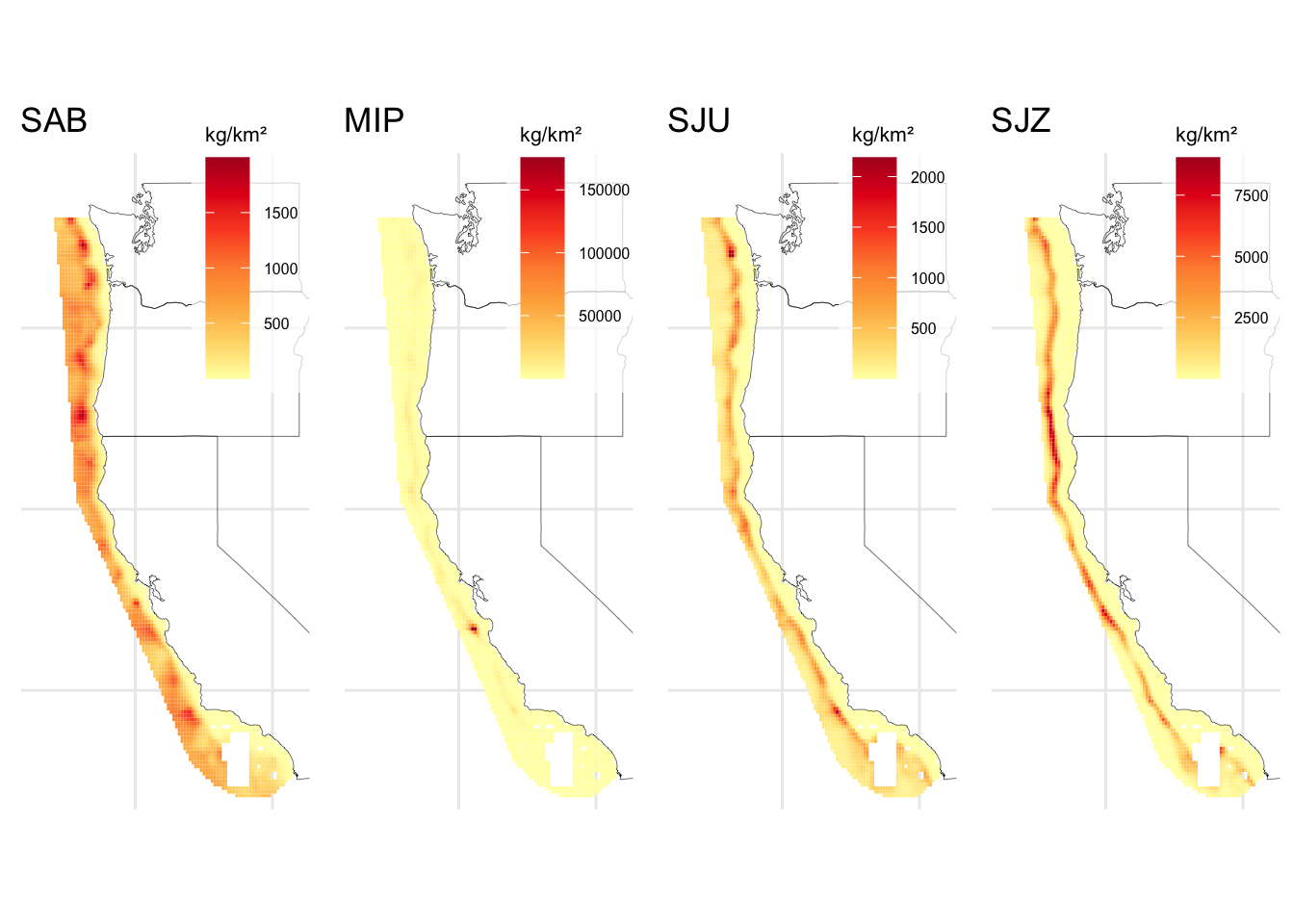
1.3 Species distribution

In this section, we will generate the population distribution needed in POPULATIONS/SpatialLayers to run DISPLACE. DISPLACE can ingest biomass density on any unit and at a continuous scale. Therefore, using species distribution data from Liu et al. (2023), we’ll spatially join it to a grid of interest and export it to a shapefile with the input formatting as detailed in Table 1.14, with GRIDCODE containing the biomass density values.

Table 1.14: Sample of the structure of the shapefile containing the species distributioin values

idx	fao_code	GRIDCODE	x
0	SAB	424.3856	POLYGON ((-119.35 32.05, -1…
0	SAB	386.2080	POLYGON ((-119.25 32.05, -1…
0	SAB	353.0033	POLYGON ((-119.15 32.05, -1…
0	SAB	317.0813	POLYGON ((-119.05 32.05, -1…
0	SAB	302.6207	POLYGON ((-118.95 32.05, -1…
0	SAB	335.1042	POLYGON ((-118.85 32.05, -1…

Figure 1.1: Species distribution in a continous scale from mean biomass values (kg/km2).

1.4 Stock abundances at szgroup

The units in the Stock_abundances_at_szgroup.csv file represent the number of individuals. DISPLACE is designed to process a specific number of length bins (0:13). Therefore, we need to adapt them based on the largest size bin for which we have abundance information (i.e., 80 cm for sablefish). The length bins will then be 6 cm.

To get these abundance values, we’ll use the catch distribution from the scientific surveys done for the stock assessments. These surveys give us the proportion of the total abundance by size group. We’ll then apply this to the yearly biomass values from the stock assessment’s modeled total biomass. After that, we’ll transform the biomass values into the number of fish using the length-weight relationship for each species. It’s worth noting that some stock assessments have a typo and weight data is in kilograms instead of grams.

The code to generate such a file is available under functions_pop.R and produces the table shown below.

stock	0	1	2	3	4	5	6	7	8	9	10	11	12	13
SAB	16321	0	0	117071.1	900204.7	2957731.7	64443823	161069586	40030449	20453968.1	3586942.8	168015.2	35788.41	1226.409
MIP	256930	0	46063450	125580385.4	67514127.9	148861830.9	342919698	170174509	33443062	925009.7	0.0	0.0	0.00	0.000
SJZ	68454	340982410	378117403	326556783.7	68729771.9	259346.3	0	0	0	0.0	0.0	0.0	0.00	0.000
SJU	13805	59005701	89485777	151768972.3	143613451.5	63939390.8	15344761	5834082	2397778	1447801.7	851419.2	210580.6	32859.72	0.000

Figure 1.2: Stock_abundances_at_szgroup.csv inout file contents.

1.4.1 Stock abundances at age

The units in the Stock_abundance_at_age.csv file are the number of individuals. DISPLACE is designed to process a specific number of age bins which is 13 (0:12), so we will have to adapt them based on our population max ages.

Common.Name	Maximum.Age	Bib.References
Sablefish	102	M. Head, Keller, and Bradburn (2014)
Shortspine Thornyhead	100	J. Zahner et al. (2023)
Longspine Thornyhead	45	Pearson and Gunderson (2003)
Dover Sole	58	Jacobson and Hunter (1993)

Figure 1.3: Detail of maximum ages.

Given a max age of 102, the bins will be 8 years. However, DISPLACE uses this to transform age into size groups. Since we already have abundance information by size from Stock_abundances_at_szgroup.csv, this table is not required. Thus, we will generate an empty table with 0s.

1.5 Stock prices data

The file Stock_prices_data.csv contains prices per kg for three length categories: small, medium, and large, for any desired currency unit. These categories can be freely defined based on the length bins. For this study case, we have defined them as follows:

Species	Size	sz_group
SAB	small	0, 1, 2, 3, 4, 5
SAB	medium	6, 7, 8, 9
SAB	large	10, 11, 12, 13
SJU	small	0, 1, 2, 3, 4, 5
SJU	medium	6, 7, 8, 9
SJU	large	10, 11, 12, 13
SJZ	small	0, 1, 2, 3, 4, 5
SJZ	medium	6, 7, 8, 9
SJZ	large	10, 11, 12, 13
MIP	small	0, 1, 2, 3, 4, 5
MIP	medium	6, 7, 8, 9
MIP	large	10, 11, 12, 13

Figure 1.4: Detail sizes grouping based on Stock_abundances_at_szgroup.csv size bins. This is used to define the species distribution .shp files as well.

To calculate stock prices, we determine the average price per kilogram for each species based on revenue data from the VMS-TIX dataset, across the entire time series.

species	rev_kg	fao_code
sablefish	6.938894	SAB
sole dover	2.138809	MIP
thornyhead longspine	2.933431	SJZ
thornyhead shortspine	6.594746	SJU

Figure 1.5: Average $/kg from fish ticket data.

Since we do not have information on price based on individual fish size, we can not categorize prices by size group. Thus we will assign the same average price to all categories and store it into the Stock_prices_data.csv.

stock	small	medium	large
SAB	6.938894	6.938894	6.938894
MIP	2.138809	2.138809	2.138809
SJZ	2.933431	2.933431	2.933431
SJU	6.594746	6.594746	6.594746

Figure 1.6: Stock_prices_data.csv input file contects.

1.6 Files overlook

Stock_biological_traits.csv:

UseIt	stock	Winf	k	Linf	CV_Linf	K	t0	a	b	L50	alpha	beta	r_age	tac_tons	fbar_age_min	fbar_age_max	F_target	F_percent	TAC_percent	B_trigger	FMSYlower	FMSYupper	FMSY	fbar_assessment	ssb_assessment	mls_cat	mls	sz_bin_cm	unit_sizebin	CV_recru	mat	mat_cat	etha_m	kappa	q	n	fzeroest	species
Yes	SAB	NA	NA	58.62105	0.090500	0.374000	-1.1883843	3.3e-06	3.27136	52.66064	NA	NA	NA	8474.875	NA	NA	0.069	0.0546881	0.0546881	NA	0.057	0.0820	0.069	0.0208000	86995	0	0	6	1	2.4696816	52.66064	9	NA	NA	NA	NA	NA	Anoplopoma fimbria
Yes	MIP	NA	NA	45.06160	0.080000	0.111500	-1.6668960	2.8e-06	3.35000	30.76170	NA	NA	NA	50000.000	NA	NA	0.130	0.0000000	0.0000000	NA	0.120	0.1300	0.130	0.0150000	221913	0	0	6	1	0.3609974	30.76170	5	NA	NA	NA	NA	NA	Microstomus pacificus
Yes	SJZ	NA	NA	28.18212	0.040000	0.108505	-0.3426386	4.3e-06	3.35200	17.82600	NA	NA	NA	3331.750	NA	NA	0.071	-0.0398461	-0.0398461	NA	0.068	0.0745	0.071	0.0236364	26771	0	0	6	1	0.6582776	17.82600	3	NA	NA	NA	NA	NA	Sebastolobus altivelis
Yes	SJU	NA	NA	95.20000	0.109034	0.013342	-7.1225000	4.8e-06	3.25500	31.40000	NA	NA	NA	2345.250	NA	NA	0.017	-0.0346059	-0.0346059	NA	0.016	0.0170	0.017	0.0091300	10135	0	0	6	1	0.5329404	31.40000	5	NA	NA	NA	NA	NA	Sebastolobus alascanus

Stock_abundances_at_szgroup.csv:

stock	0	1	2	3	4	5	6	7	8	9	10	11	12	13
SAB	16321	0	0	117071.1	900204.7	2957731.7	64443823	161069586	40030449	20453968.1	3586942.8	168015.2	35788.41	1226.409
MIP	256930	0	46063450	125580385.4	67514127.9	148861830.9	342919698	170174509	33443062	925009.7	0.0	0.0	0.00	0.000
SJZ	68454	340982410	378117403	326556783.7	68729771.9	259346.3	0	0	0	0.0	0.0	0.0	0.00	0.000
SJU	13805	59005701	89485777	151768972.3	143613451.5	63939390.8	15344761	5834082	2397778	1447801.7	851419.2	210580.6	32859.72	0.000

Stock_abundance_at_age.csv:

year	stock	0	1	2	3	4	5	6	7	8	9	10	11	12
2022	SAB	0	0	0	0	0	0	0	0	0	0	0	0	0
2022	MIP	0	0	0	0	0	0	0	0	0	0	0	0	0
2022	SJZ	0	0	0	0	0	0	0	0	0	0	0	0	0
2022	SJU	0	0	0	0	0	0	0	0	0	0	0	0	0

Stock_prices_data.csv:

stock	small	medium	large
SAB	6.938894	6.938894	6.938894
MIP	2.138809	2.138809	2.138809
SJZ	2.933431	2.933431	2.933431
SJU	6.594746	6.594746	6.594746

Adams, Grant D., Owen S. Hamel, and Ian G. Taylor. 2019. “Catch Only Update: Stock Assessment and Status of Longspine Thornyhead (Sebastolobus Altivelis) Off California, Oregon and Washington in 2019.” Seattle, Washington: School of Aquatic; Fishery Sciences, University of Washington; Northwest Fisheries Science Center, U.S. Department of Commerce, National Oceanic; Atmospheric Administration, National Marine Fisheries Service. https://www.pcouncil.org/documents/2019/09/agenda-item-h-5-supplemental-revised-attachment-23.pdf/.

Blanchard, Julia L, Ryan F Heneghan, Jason D Everett, Rowan Trebilco, and Anthony J Richardson. 2017. “From Bacteria to Whales: Using Functional Size Spectra to Model Marine Ecosystems.” Trends in Ecology & Evolution 32 (3): 174–86. https://doi.org/10.1016/j.tree.2016.12.003.

Fay, G. 2005. “Stock Assessment and Status of Longspine Thornyhead (Sebastolobus Altivelis) Off California, Oregon and Washington in 2005.” Portland, Or: PFMC. https://www.pcouncil.org/documents/2020/12/stock-assessment-and-status-of-longspine-thornyhead-sebastolobus-altivelis-off-california-oregon-and-washington-in-2005-august-30-2005.pdf/.

Guzmán, José M, J Adam Luckenbach, Mollie A Middleton, Kenneth C Massee, Cortney Jensen, Frederick W Goetz, Andrew J Jasonowicz, and Penny Swanson. 2017. “Reproductive Life History of Sablefish (Anoplopoma Fimbria) from the US Washington Coast.” Plos One 12 (9): e0184413. https://doi.org/10.1371/journal.pone.0184413.

Haltuch, MA, KF Johnson, N Tolimieri, MS Kapur, and CA Castillo-Jordán. 2019. “Status of the Sablefish Stock in u.s. Waters in 2019.” 7700 Ambassador Place NE, Suite 200, Portland, OR: Pacific Fisheries Management Council. https://www.pcouncil.org/documents/2019/10/status-of-the-sablefish-stock-in-u-s-waters-in-2019-october-22-2019.pdf/.

Haltuch, Melissa A., Kelli F. Johnson, Nick Tolimieri, Maia S. Kapur, and Claudio A. Castillo-Jordán. 2019. “Status of the Sablefish Stock in u.s. Waters in 2019.” Seattle, WA, USA: National Marine Fisheries Service, Northwest Fisheries Science Center. https://www.pcouncil.org/documents/2019/10/status-of-the-sablefish-stock-in-u-s-waters-in-2019-october-22-2019.pdf/.

Head, MA, AA Keller, and M Bradburn. 2014. “Maturity and Growth of Sablefish, Anoplopoma Fimbria, Along the US West Coast.” Fisheries Research 159: 56–67. https://doi.org/10.1016/j.fishres.2014.05.007.

Head, Melissa A, Aimee A Keller, and Mark Bradburn. 2014. “Maturity and Growth of Sablefish, Anoplopoma Fimbria, Along the US West Coast.” Fisheries Research 159: 56–67. https://doi.org/10.1016/j.fishres.2014.05.007.

Hunter, John R., John L. Butler, Carol Kimbrell, and Eric A. Lynn. 1990. “Bathymetric Patterns in Size, Age, Sexual Maturity, Water Content, and Caloric Density of Dover Sole, *Microstomus Pacificus*.” CalCOFI Investigative Reports 31: 132–44. https://calcofi.com/publications/calcofireports/v31/Vol_31_Hunter_etal.pdf.

Jacobson, LD, and JR Hunter. 1993. “Bathymetric Demography and Management of Dover Sole.” North American Journal of Fisheries Management 13 (3): 405–20.

Johnson, Kelli F., Chantel R. Wetzel, and Nick Tolimieri. 2023. “Status of Sablefish (Anoplopoma Fimbria) Along the u.s. West Coast in 2023.” 2725 Montlake Boulevard East, Seattle, Washington 98112: Northwest Fisheries Science Center, U.S. Department of Commerce, National Oceanic; Atmospheric Administration, National Marine Fisheries Service. https://www.pcouncil.org/documents/2024/02/status-of-sablefish-anoplopoma-fimbria-along-the-u-s-west-coast-in-2023.pdf/.

Liu, Owen R, Eric J Ward, Sean C Anderson, Kelly S Andrews, Lewis AK Barnett, Stephanie Brodie, Gemma Carroll, et al. 2023. “Species Redistribution Creates Unequal Outcomes for Multispecies Fisheries Under Projected Climate Change.” Science Advances 9 (33): eadg5468. https://www.science.org/doi/full/10.1126/sciadv.adg5468.

Pacific Fishery Management Council. 2016. “2017-2018 Groundfish Harvest Specifications and Management Measures Including Changes to Groundfish Stock Designations (Amendment 27 to the Pacific Coast Groundfish Fishery Management Plan): Description and Analysis for Council Decision-Making.” Report. Suite 101, 7700 NE Ambassador Place, Portland, OR 97220: Pacific Fishery Management Council. https://www.pcouncil.org/documents/2016/09/2017-2018-groundfish-harvest-specifications-and-management-measures-analytical-document-revised.pdf/.

———. 2018. “Pacific Coast Groundfish Fishery 2019–20 Harvest Specifications, Yelloweye Rebuilding Plan Revisions, and Management Measures.” Report. 7600 Sand Point Way NE, Seattle, WA 98115: Pacific Fishery Management Council. https://www.pcouncil.org/documents/2020/12/final-environmental-assessment-magnuson-stevens-act-analysis-regulatory-impact-review-regulatory-flexibility-act-analysis-pacific-coast-groundfish-fishery-2019-20-harvest-specifications-yelloweye-re.pdf/.

———. 2020. “Preferred 2021 and 2022 Harvest Specifications, Acceptable Biological Catches, and Annual Catch Limits for West Coast Groundfish Stocks and Stock Complexes Under Preferred Harvest Specifications.” Report. Suite 101, 7700 NE Ambassador Place, Portland, OR 97220: Pacific Fishery Management Council. https://www.pcouncil.org/documents/2020/05/f-1-attachment-7-preferred-2021-and-2022-harvest-specifications-acceptable-biological-catches-and-annual-catch-limits-for-west-coast-groundfish-stocks-and-stock-complexes-under-preferred-harvest-c.pdf/.

———. 2022. “Pacific Coast Groundfish Fishery 2023-2024 Harvest Specifications and Management Measures: Draft Analytical Document, the Preferred Alternative.” Report. Suite 101, 7700 NE Ambassador Place, Portland, OR 97220: Pacific Fishery Management Council. https://www.pcouncil.org/documents/2022/08/draft-management-measure-analytical-document-the-preferred-alternative-september-2022.pdf/.

Pearson, KE, and DR Gunderson. 2003. “Reproductive Biology and Ecology of Shortspine Thornyhead Rockfish, Sebastolobus Alascanus, and Longspine Thornyhead Rockfish, s. Altivelis, from the Northeastern Pacific Ocean.” Environmental Biology of Fishes 67: 117–36.

Rodgveller, Cara J., James W. Stark, and Katy B. Echave. 2016. “Age at Maturity, Skipped Spawning, and Fecundity of Female Sablefish (Anoplopoma Fimbria) During the Spawning Season.” Fishery Bulletin 114 (1): 89–102. https://repository.library.noaa.gov/view/noaa/12546.

Stephens, A, and IG Taylor. 2013. “Stock Assessment and Status of Longspine Thornyhead (Sebastolobus Altivelis) Off California, Oregon and Washington in 2013.” Portland, Or: PFMC. https://www.pcouncil.org/documents/2014/02/stock-assessment-and-status-of-longspine-thornyhead-sebastolobus-altivelis-off-california-oregon-and-washington-in-2013-published-january-5-2014.pdf/.

Stockhausen, William T., Benjamin J. Turnock, Z. Teresa A’mar, Mark E. Wilkins, and Michael H. Martin. 2005. “4a. Gulf of Alaska Dover Sole.” https://apps-afsc.fisheries.noaa.gov/refm/docs/2005/GOAdover.pdf.

Wetzel, Chantel R., and Aaron M. Berger. 2021. “Status of Dover Sole (Microstomus Pacificus) Along the u.s. West Coast in 2021.” Seattle, Washington; Newport, Oregon: Northwest Fisheries Science Center, U.S. Department of Commerce, National Oceanic; Atmospheric Administration, National Marine Fisheries Service. https://www.pcouncil.org/documents/2021/10/status-of-dover-sole-microstomus-pacificus-along-the-u-s-west-coast-in-2021.pdf/.

Zahner, JA, MA Heller-Shipley, HA Oleynik, SG Beyer, P-Y Hernvann, M Véron, AN Odell, et al. 2023. “Status of Shortspine Thornyhead (Sebastolobus Alascanus) Along the US West Coast in 2023.” Portland, Oregon: Pacific Fishery Management Council.

Zahner, Joshua A., Madison Heller-Shipley, Haley A. Oleynik, Sabrina G. Beyer, Pierre-Yves Hernvann, Matthieu Véron, Andrea N. Odell, et al. 2023. “Status of Shortspine Thornyhead (Sebastolobus Alascanus) Along the US West Coast in 2023.” Seattle, Washington; Vancouver, British Columbia; Santa Cruz, California; Davis, California; Juneau, Alaska: School of Aquatic; Fishery Sciences, University of Washington; Institute for the Oceans; Fisheries, University of British Columbia; Institute of Marine Sciences’ Fisheries Collaborative Program, University of California-Santa Cruz; Northwest Fisheries Science Center, U.S. Department of Commerce, National Oceanic; Atmospheric Administration, National Marine Fisheries Service; Alaska Fisheries Science Center, U.S. Department of Commerce, National Oceanic; Atmospheric Administration, National Marine Fisheries Service; University of California Davis. https://www.pcouncil.org/documents/2024/02/status-of-shortspine-thornyhead-sebastolobus-alascanus-along-the-us-west-coast-in-2023.pdf/.